Learning CFD with OpenFOAM and Linux
Table of Contents
- 1. How to install Linux and OpenFOAM
- 2. First steps in your new Linux environment
- 3. Setting up your first case
- 4. Accessing the Linux Filesystem in WSL2 from Windows
- 5. Installing Extras and Additional Solvers
- 6. OpenFOAM directory conventions
- 7. OpenFOAM Boundary Conditions
- 8. Cluster Access
1. How to install Linux and OpenFOAM
1.1. Which version of OpenFOAM?
There are a few different versions of OpenFOAM, which are related, but have separated along the way. All of them are similar, and many of the principles will be the same, but they differ in detail, so a solver or case set up for one variant may not work in the other (but it is usually possible to convert them).
- OpenFOAM.org - released by the OpenFOAM foundation. Version numbers are of the form N. Current release is OpenFOAM 8. The release cycle is irregular.
- OpenFOAM.com - released by ESI. Version numbers are of the form vYYMM, where YY is the year and MM the month of the release. Current version is v2106, released in June 2021. The release cycle is 6 months. This variant is popular with commercial users, since the copyright of derived code does not need to be transferred to ESI. This variant also has - in my opinion - the most extensive documentation.
These two variants are quite close and most settings are the same. Adaptations of cases from one to the other is usually straightforward. But the feature set is different and more current models may be available in one, but not the other.
- foam-extend, released by a loose-knit group of developers, led by Hrvoje Jasak. This is a variant that has been forked from the original codebase and has a quicker way for new models to be integrated. On the other hand it is more fluid and chaotic. This is the most difficult to get used to.
Usually I would recommend you to start with the version that is most easily installed on your system. This would be either OpenFOAM 8 or OpenFOAM v2106.
1.2. Which system to run it on?
1.2.1. Linux
OpenFOAM is Linux software. So the best option would be to run it on a Linux system. There are many different variations of Linux out there, so called distributions. The one distribution I would recommend for a beginner (and which we will use in one form or the other) is Ubuntu because it is currently the most popular and is (in my view) the easiest to install. Another reason is that OpenFOAM is available as an installation package for this distribution.
Linux can be installed on most machines, so if you have a computer that has enough room on a hard drive (or you have a spare hard drive) you can install Linux alongside the Windows system in a so-call “dual-boot” configuration, where you can select the operating system in a boot menu. Ubuntu comes as a bootable image that you can put on a usb drive and boot from it. The cool thing is that that image is a “live system”, so you can boot into Ubuntu directly from the usb-drive and test the system before you install it. Select the option to install it alongside the existing Windows installation and the installer will do the rest1.
1.2.2. Windows WSL2
To run OpenFOAM on Windows you can use Windows Subsystem for Linux (WSL2) which comes with Windows 10. In WSL2 you can then install a Linux system (Ubuntu 20.04LTS) and then run OpenFOAM in that. Detailed instructions on the Microsoft website. Follow these and select Ubuntu 20.04LTS as the Linux distribution to install2. On some systems you will need to activate the virtualisation in the BIOS3 See this page - on AMD systems the setting may also be called AMD-V.
1.2.3. Windows Docker
You can also install a docker image containing both Linux and OpenFOAM. This requires you to install docker and then install a docker image with a Linux system and OpenFOAM.
This is an interesting method, but I have not tested it. You may want to give it a go. Please let me know and we can try that. On Windows the docker container runs in a small virtual box, so it may have some performance penalty over WSL2.
1.2.4. Run Linux on an Azure Labs remote desktop
The university has a subscription to Azure Labs from Microsoft. Azure is a remote desktop system, so you can run everything in the cloud through your browser. This is an excellent solution if your computer is not fast enough or does not have enough RAM to run OpenFOAM directly. It should even work on a Chromebook. We are currently finalising the setup, and I will update this entry with the details.
1.3. First steps…
Once you have Ubuntu installed, it would be a good time to get to know your new system and take the first steps in Ubuntu. If you installed in WSL2 you will not need the bit about the GUI, since you will only be using the terminal. After you have familiarised yourself with the system, you can continue here:
1.4. Installing OpenFOAM in Ubuntu
Regardless of which system setup you chose, you will need to install OpenFOAM in the Linux system. If you have installed Ubuntu in the WSL2 you should have an “Ubuntu” icon somewhere - find it and start this, it should open a shell.
Installation of software in Ubuntu is done using the package manager. For packages that are known to the package manager, i.e. that reside in repositories included with Ubuntu, the installation is done using the command:
apt install packagename
You will need to decide, which version of OpenFOAM you will use4. I will use OpenFOAM v2106 for most of the examples, and have tested my software with that release. If you plan on using solids4Foam5, then I recommend to use OpenFOAM v7, since that is the one that is tested for that extension.
1.4.1. OpenFOAM v2106
OpenFOAM v2106 is the ESI version of OpenFOAM. You can also use their Installation Instructions. It is not in an included repository, so before you can install it you need to add the repository and the security keys:
curl -s https://dl.openfoam.com/add-debian-repo.sh | sudo bash
Simply copy and paste the above line into the terminal. This runs a script that will add the repository to your system configuration. After that you can install the OpenFOAM packages using:
    sudo apt update
    sudo apt install openfoam2106-default
To initialise OpenFOAM, you open a terminal and type:
openfoam2106
1.4.2. OpenFOAM 7
OpenFOAM 7 is the Foundation version of OpenFOAM6. You can also use their Installation Instructions.
sudo sh -c "wget -O - https://dl.openfoam.org/gpg.key | apt-key add -"
sudo add-apt-repository http://dl.openfoam.org/ubuntu
Simply copy and paste the above line into the terminal. This runs a script that will add the repository to your system configuration. After that you can install the OpenFOAM packages using:
    sudo apt update
    sudo apt install openfoam7
This will install version 7 of Foundation-OpenFOAM. If you want to install the newest version as well (not required):
sudo apt install openfoam9
To initialise OpenFOAM 7, you open a terminal and type:
source /opt/openfoam7/etc/bashrc
2. First steps in your new Linux environment
When you boot up your new Linux environment, you will be greeted by the Desktop Environment (DE). The DE is the graphical user interface on top of the Operating System (OS). One of the most prominent features of Linux as on OS is, that there is no “Linux”. Linux is the common name for a lot of different distributions, each of which has their own special features. When you enter “Best Linux Distribution” into a search engine, you’ll find a lot of conflicting answers, because the question is wrong7. There is no best distribution, because everybody expects different things from their computer system. The distribution I use for most of my computing needs is Ubuntu8, since it is easy to install, is robust, has a dependable update cycle, is popular - so most software will have a package that is easy to install, and has a really good community to get help, if you need it.
The same can be said for the Desktop Environment. There are many different desktop environments and all are different. Two more prominent ones are GNOME and KDE, but there are many others, and it is a matter of preference, what you choose. In some of the screencast that I will record you will see that I use a rather niche DE: regolith which is mainly keyboard driven - I don’t recommend that for beginners, but you may wonder why my screens look so weird8.
On a standard Ubuntu Installation the DE will be a GNOME 3 desktop. On the Azure Remote Desktop you will get a DE that is less demanding on the graphics (and thus will run better over the remote desktop link): XFCE.
2.1. Getting to know the Desktop Environment
The DE will look more or less familiar, GNOME will be somewhere between MacOS and Windows9, while XFCE will be closer to the typical Windows experience.
Have a look at the help for the DE you are using: -
On Ubuntu/GNOME you can also click the little Lifesaver icon in the side panel. Play around with it for a while. You will soon get used to it. It’s only difficult because it’s different to what you are used to - I’ve upgraded my mother’s Windows 7 machine to Ubuntu and she says, it’s easier to use (and a lot faster).
2.2. In the beginning was the command line10 …
What my mother does not need to do, but you will have to, is use the command line. In the age of touch screens, where some people think keyboards are archaic, this will be a major hurdle for many.
But the command line is “an elegant weapon from a more civilised age”, and far from obsolete11. In a “tourist in a shop” language analogy, a graphical user interface is like grunting and pointing, whereas the command line is speaking a language fluently.
With some practice the command line will allow you to work on the computer faster than a graphical interface can. The only problem is, you have to learn a language: have a look at this introduction course, and then go to linuxcommand.org and download the book.
3. Setting up your first case
3.1. Test the installation
Lets set up FOAM for the first case. Simply type, or copy and paste the commands one by one into the shell - remember the highlight and middle mouse trick from the command line tutorials?
initialise OpenFOAM:
openfoam2106
create the case directory:
    mkdir -p $FOAM_RUN

    run
the last command changes to the case (or run) directory, which is usually located at /home/username/OpenFOAM/username-v2106/run - username is your username, v2006 is the OpenFOAM version. Alternatively you can change into this directory with (from the home directory):
cd OpenFOAM/username-v2106/run
There are many tutorials that come with OpenFOAM. Let’s copy one and run it:
    cp -r $FOAM_TUTORIALS/incompressible/icoFoam/elbow $FOAM_RUN/
    cd $FOAM_RUN/elbow
    ls
this will output something like
0 Allclean Allrun constant elbow.msh system
The directories and files that you see here are:
0: This contains the start and boundary conditions (0 is the zeroth timestep/iteration). Once the case is run the results will also be in directories that are named with the time or number of iterations, e.g.1000after 1000 iterations for steady state, or2.5after 2.5 seconds.constant: Here are the files that define the constants, like fluid properties, mesh, etc.system: In this directory you will find the system/solver settings. Most importantly the filecontrolDictthat has all the main settings,fvSchemeswith the discretisation schemes, andfvSolutionwith the solver settings, like internal iterations, convergence criteria, and such.elbow.mshis a Fluent mesh file. This is the same case as the first Fluent tutorial, the mixing elbow. We have stolen the mesh from there ;-)AllrunandAllcleanare scripts that run the case and “cleanup” the directory, i.e. delete all the results (be careful with the Allclean script!).
You can simply run the case now by typing ./Allrun (the ./ is required to run programs or scripts in the current directory). But that wouldn’t teach us a lot. So let’s have a look at this file:
Open the file in your text editor, or type:
less Allrun
You remember less from the command line tutorials, don’t you?
This will show you:
#!/bin/sh
cd "${0%/*}" || exit                                # Run from this directory
. ${WM_PROJECT_DIR:?}/bin/tools/RunFunctions        # Tutorial run functions
#------------------------------------------------------------------------------

restore0Dir

runApplication fluentMeshToFoam \
    ${FOAM_TUTORIALS:?}/resources/geometry/elbow.msh

runApplication $(getApplication)

runApplication foamMeshToFluent

runApplication foamDataToFluent

#------------------------------------------------------------------------------
This is a shell script which runs four commands: fluentMeshToFoam, which converts a Fluent mesh to a FOAM mesh (who would have guessed with that name!); then the solver is run, $(getApplication) looks up the application to run in the system/controlDict file; then the next two would convert the mesh foamMeshToFluent and results foamDataToFluent back to the Fluent format (and write a .cas and a .dat file) in order to be postprocessed in Fluent. But we won’t need those, since you will use Paraview to visualise the results.
So we can convert the Fluent mesh (which is in another directory, so you’ll need the call it using a weird path) and run the solver with:
    fluentMeshToFoam ${FOAM_TUTORIALS:?}/resources/geometry/elbow.msh

    icoFoam
3.2. Have a look at the data with ParaView
3.2.1. If you run it on WSL2:
You will have to install Paraview on the Windows system.
Then you need to create an empty file called casename.foam in the case directory. The easiest way to do that is:
touch casename.foam
This is a file that will tell ParaView to read the data directly from the FOAM file structure.
Then you can open Paraview and open that file from the “File” menu. But before you can do that, you will need to set up access to the Linux Filesystem in WSL2 from Windows (below).
3.2.2. If you run it on Linux:
Then we can open ParaView using the command:
paraFoam
This is a command that sets up the case to be read in ParaView and then calls ParaView.
Oops, something went wrong? What’s the error message?
    Cannot use ParaView reader module library (PVFoamReader)
    The PV_PLUGIN_PATH environment value is not set

    Continuing with builtin reader:  paraFoam -vtk

    Created temporary 'elbow.foam'
    /opt/openfoam/openfoam7/bin/paraFoam: 327: paraview: not found
The first is not an error, it can’t use one reader, but falls back to the builtin one, that’s fine. The error is paraview: not found.
So we need to install that first. Luckily that’s easy on a Ubuntu system:
sudo apt install paraview
will download and install ParaView and automatically download and install a lot of other packages that ParaView depends on.
You can start Paraview with:
paraFoam
and have a look at the data. Information about Paraview can be found on the ParaView website. Have a look under “Resources”.
Have fun. You may want to have a look at some of the other tutorials as well.
We will have a closer look at the anatomy of OpenFOAM cases soon. In the meantime check the user guide.
4. Accessing the Linux Filesystem in WSL2 from Windows
WSL makes the Linux filesystem accessible from Windows in the form of a network drive.
The network address for your home directory is of the form
\\wsl$\distributionName\home\userName
The easiest way to make this available to, e.g. ParaView, is the following:
- Open the windows file manager
- Click into the address bar (to the right of the current path), this will change the address bar into a text entry field.
- Delete the path that’s in there, and enter
\\wsl$and confirm - Then click through to the folder containing your home directory
\\wsl$\Ubuntu-20.04\home - Create a shortcut on the Desktop (or wherever you prefer) by dragging
this home directory to the desktop while holding the
ALTkey.
You can now access all the files in your Linux home directory in Windows applications. E.g. in order to have a look at the data with ParaView or edit the OpenFOAM files with a Windows text editor12.
5. Installing Extras and Additional Solvers
5.1. Install haemoFoam and PyFOAM
The biomedical code that you will use is not part of OpenFOAM, but has been written by me, using the OpenFOAM framework. You will have to install this code in your user OpenFOAM directory.
While we are at it, we will also install Python and PyFOAM, which provides
useful tools for managing OpenFOAM cases.
5.1.1. Install Python and PyFOAM
Python is an object-oriented programming and scripting language that is widely used in data and engineering science. In is often used to control computational systems, as well. We will use PyFOAM, which is a set of utilities for OpenFOAM which make case handling and setup easier.
5.1.1.1. Update Ubuntu
    sudo apt -y update

    sudo apt -y upgrade

    sudo apt -y dist-upgrade
This will upgrade all packages in your Ubuntu installation and may take a while.
5.1.1.2. and install Python and some other things:
    sudo apt -y install python3 python3-pip python3-dev python3-scipy python3-pandas python-is-python3

    sudo apt -y install rpm curl libopenmpi-dev libreadline-dev dstat
5.1.1.3. then install PyFOAM:
pip3 install --user PyFOAM
5.1.2. Install haemoFOAM
HaeoFoam is the code that I wrote for blood flow simulations. It is written in
C++ using the OpenFOAM framework and includes some additional features:
- non-Newtonian rheology models, in particular the Quemada model Quemada1977,Quemada1978,Quemada1978b and a modified Krieger-Dougherty model Hund2017, as well as the original Krieger model Krieger1959,Woods1970,Papir1970.
- haematocrit transport model based on Phillips1992.
- windkessel boundary conditions Westerhof2009, adapted from code written by colleagues at Imperial College, London Piebalgs2017,Piebalgs2018,Pirola2017
haemoFoam is hosted on github, and if you have a github account and know how to
compile code, I can give you access to it. But to make things easier, I have
precompiled this code for you and you can simply download an archive file
OF2106_apps.tgz from the projects Google Drive, move it to the Linux filesystem
(into your home directory) (see How to access the Linux file system from
Windows) and then install it as follows:
    cd ~/OpenFOAM/$USER-v2106/
    tar xvfz ~/OF2106_apps.tgz
Test that the installation worked with:
Initialise OpenFOAM (unless already initialised):
openfoam2106
Call a haemoFOAM solver:
haemoPimpleFoam
This should output something like:
    /*---------------------------------------------------------------------------*\
    | =========                 |                                                 |
    | \\      /  F ield         | OpenFOAM: The Open Source CFD Toolbox           |
    |  \\    /   O peration     | Version:  v2106                                 |
    |   \\  /    A nd           | Website:  www.openfoam.com                      |
    |    \\/     M anipulation  |                                                 |
    \*---------------------------------------------------------------------------*/
    Build  : 14410a73-20200806 OPENFOAM=1912 patch=200727
    Arch   : "LSB;label=32;scalar=64"
    Exec   : haemoPimpleFoam
    Date   : Oct 31 2020
    Time   : 16:27:12
    Host   : TS-ZBook-17
    PID    : 2860549
    I/O    : uncollated
    Case   : /home/acests3/OpenFOAM/acests3-v1912
    nProcs : 1
    trapFpe: Floating point exception trapping enabled (FOAM_SIGFPE).
    fileModificationChecking : Monitoring run-time modified files using timeStampMaster (fileModificationSkew 10)
    allowSystemOperations : Allowing user-supplied system call operations

    // * * * * * * * * * * * * * * * * * * * * * * * * * * * * * * * * * * * * * //
    Create time


    --> FOAM FATAL ERROR:
    cannot find file "/home/acests3/OpenFOAM/acests3-v1912/system/controlDict"

        From function virtual Foam::autoPtr<Foam::ISstream> Foam::fileOperations::uncollatedFileOperation::readStream(Foam::regIOobject&, const Foam::fileName&, const Foam::word&, bool) const
        in file global/fileOperations/uncollatedFileOperation/uncollatedFileOperation.C at line 548.

    FOAM exiting
It fails, since there is no case file to run, but if you see the header file, then the installation was successful and your system is ready for the project.
6. OpenFOAM directory conventions
In order to work efficiently with OpenFOAM we have to understand the file system structure of OpenFOAM itself and of OpenFOAM cases.
Make sure you understand the basics of Linux/Unix file systems and have mastered basic Linux commands given in the tutorial before doing any of the advanced work.
6.1. Your home directory
Your home directory is placed in /home/userName, where userName is your user name on the system (chosen at installation or when creating the user. Every user of a Linux system will have their own home directory.
The home directory has a shortcut, which is the “tilde” character ~
You can change to your home directory with:
cd
That is, the cd command without any argument, or
cd ~
You can also use the ~ to refer to the home directory in most commands:
cd ~/OpenFOAM
will change into the OpenFOAM directory in your home directory from wherever you are.
6.2. The OpenFOAM directories
OpenFOAM has its own directory structure, which looks like this:
OpenFOAM
├── userName-v2106
│   ├── applications
│   ├── platforms
│   ├── run
where userName is your username.
The userName-v2106 (for version 21.06 of OpenFOAM, if you have more than one version installed, you may have more than one of these directories) is the base.
In that you have:
applicationscontaining your own code. Most of you won’t need that until you start writing your own solvers or libraries, e.g. for boundary conditions.platformscontains the compiled executables and libraries of the code inapplications. On your system that should contain two directoriesbinandlibcontaining the libraries forhaemoFOAMandswak4FOAM, (SWiss Army Knife 4 FOAM) an extension to OpenFOAM, that provides, amongst other things the Groovy Boundary Condition,groovyBC, that we are going to use.run, the directory where you should keep your cases. While the former two directories have to be in their fixed locations, you can run cases in any directory you like, but this one is the recommended one.
6.3. OpenFOAM case structure
Typically OpenFOAM will be located in the run directory above. You can, however, place them anywhere on the file system (only where you have write access, of course), e.g. if your system has a workspace for larger cases (many cluster systems will have such a directory).
The important thing is that the case is a collection of files that are in a directory structure. This means that there is no single file that you can copy, but you need to copy the whole directory. This can be done by archiving the case using either the Linux command tar, or (if you need to use the case on a Windows system) the zip command, or by creating an archive using the pyFoamArchive.py command (this will also delete most of the results, so use with care).
A case named casename will have a structure like this:
casename
├── 0
├── constant
├── casename.foam
└── system
0, constant=, and system are directories that contain:
0: initial conditions and boundary conditions are described by files in this directory. See OpenFOAM Boundary Condition Files. The0directory is the first (zero-th) of the time directories. The other time directories will contain the results and are named by theirrunTime, i.e. a directory named1.5will contain the result after 1.5 seconds.constant: contains the parameters and settings that remain constant throughout the run. This will be the physical parameters for the fluid (or solid), turbulence models, etc. This directory will also contain the (initial) mesh in thepolyMeshsub-directory.system: contains the controlling files, most importantlycontrolDict.
Also see OpenFOAM User Guide: 2.1 File Structure of OpenFOAM cases
7. OpenFOAM Boundary Conditions
7.1. Initial and Boundary Conditions
Since CFD is a numerical integration method, we will need to define initial (IC) and boundary conditions (BC) for the integration in time and space, respectively. Initial and boundary conditions must be provided for all components of the solution vector - in the minimal case pressure p and velocity vector U, haemoFOAM also needs IC and BC for haematocrit concentration H.
Both initial and boundary conditions are set in the files in the time directories, in particular the 0 directory. Please also refer to the official documention for the file structure of OpenFOAM cases, and the Youtube Video - Setting up out First Case.
The 0 directory contains the files H, p, and U, for haematocrit, pressure, and velocity vector, respectively:
  ~/OpenFOAM/acests3-v1912/run/carotid_steadyState_template
  ❯ ls 0
  H  p  U
7.2. Anatomy of IC/BC files
Please also see the official documentation, which is quite brief, so I’ll expand on it here.
The IC/BC files look like this:
/*--------------------------------*- C++ -*----------------------------------*\
| =========                 |                                                 |
| \\      /  F ield         | OpenFOAM: The Open Source CFD Toolbox           |
|  \\    /   O peration     | Version:  v1912                                 |
|   \\  /    A nd           | Website:  www.openfoam.com                      |
|    \\/     M anipulation  |                                                 |
\*---------------------------------------------------------------------------*/
FoamFile
{
    version     2.0;
    format      ascii;
    class       volVectorField;
    object      U;
}
// * * * * * * * * * * * * * * * * * * * * * * * * * * * * * * * * * * * * * //

dimensions      [0 1 -1 0 0 0 0];

internalField   uniform (0 0 0);

boundaryField
{
    inlet
    {
        type            fixedValue;
        value           uniform (10 0 0);
    }

    outlet
    {
        type            zeroGradient;
    }

    upperWall
    {
        type            noSlip;
    }

    lowerWall
    {
        type            fixedValue;
        value           uniform (0 0 0);
    }

    frontAndBack
    {
        type            empty;
    }
}

// ************************************************************************* //
The first 7 lines are comments which are mostly decorative (the file will still work without them). The first line has a *- C++ -* in the middle which will tell most editors to use C++ mode - not strictly needed, but useful.
The next 7 lines are important and tell OpenFOAM what the contents are and how to read them:
  FoamFile
  {
      version     2.0;
      format      ascii;
      class       volVectorField;
      object      U;
  }
This block is always of the form FoamFile{ }. The version is the configuration file version, not the OpenFOAM version. This is very stable and has not changed for a long time. Most OpenFOAM cases can easily be opened and run on different versions of FOAM, unlike most commercial CFD packages, which tend not to be backward compatible. The file format is usually ascii, i.e. plain text. Keep all file formats in ascii for compatibility and easy of use, since they will always be human readable then.
The next two lines are the important ones. They tell the system that the file contains a vector field stored in the cell volumes, and the name of the “object”, in this case the velocity vector U.
All lines in C++ need to be terminated with a semicolon, forgetting the semicolon is one of the most common mistakes while editing OpenFOAM files!
7.2.1. Dimensions
The dimensions line tells the code what the dimensions of the object are. The numbers denote the exponent in the SI system in the order of:
[kg m s K mol A cd]
This means that the velocity has:
dimensions [0 1 -1 0 0 0 0];
i.e. \(m^1 s^{-1}\).
7.2.2. Initial conditions
The next line describes the initial conditions. In most cases it will be enough to initialise with a uniform value as is done here:
internalField uniform (0 0 0);
This initialised the whole field with zero velocity.
7.2.3. Boundary conditions
The rest of the file contains the boundary conditions, in a nested block:
     boundaryField
     {
       patchName
         {
           type            boundaryConditionType;
           value           boundaryConditionValues;
         }
     }
Make sure that you keep track of the opening and closing curly brackets.
We will discuss the different boundary condition types here: OpenFOAM BCs. A full list of all available boundary conditions (most of which will not be of interest in our context) can be found here.
7.3. Boundary condition types
Boundary conditions can be of two principal types:
- Value boundary conditions, where the value of the property at the boundary is set to a specified value. These are called Dirichlet boundary conditions. One example for the Dirichlet boundary conditions is the no-slip wall boundary condition, which sets the velocity to zero.
- Gradient boundary conditions, where the gradient of a value is set to a specific value. These are called Neumann boundary conditions. An example is the velocity condition at an outlet, which is commonly given as a zero gradient in velocity.
- There are combinations of these two types in the Cauchy and Mixed boundary condition.
All of the special boundary conditions are derived from these fundamental types.
In CFD the solution vector consists of pressure p and velocity U. So we have to give boundary conditions for these two properties.
In this document I will only describe the BCs we use, a full list of all available boundary conditions (most of which will not be of interest in our context) can be found here. The anatomy of an OpenFOAM boundary condition file is described here: OpenFOAM Boundary Condition Files.
7.3.1. Pressure Boundary Conditions
Most common pressure boundary conditions used in our simulations are:
- fixedValue: set boundary condition to a fixed value (very often zero relative pressure at an outlet 13)
- zeroGradient: this is the typical pressure BC that goes with a velocity BC that prescribes a fixed value for the velocity.
Windkessel boundaries are a special case, so see the Windkessel boundary documentation: Windkessel BCs
/*--------------------------------*- C++ -*----------------------------------*\
| =========                 |                                                 |
| \\      /  F ield         | foam-extend: Open Source CFD                    |
|  \\    /   O peration     | Version:     4.0                                |
|   \\  /    A nd           | Web:         http://www.foam-extend.org         |
|    \\/     M anipulation  |                                                 |
\*---------------------------------------------------------------------------*/
FoamFile
{
    version     2.0;
    format      ascii;
    class       volScalarField;
    location    "0";
    object      p;
}
// * * * * * * * * * * * * * * * * * * * * * * * * * * * * * * * * * * * * * //

dimensions      [0 2 -2 0 0 0 0];

internalField   uniform 0;

boundaryField
{
    ICA
    {
        type            fixedValue;
        value           uniform 0;
    }
    ECA
    {
        type            fixedValue;
        value           uniform 0;
    }
    wall
    {
        type            zeroGradient;
    }
    APEX
    {
        type            zeroGradient;
    }
    SINUS
    {
        type            zeroGradient;
    }
    CCA
    {
        type            zeroGradient;
    }
}
// ************************************************************************* //
Important: OpenFOAM uses kinematic pressures, not static pressures. Note that the dimensions [0 2 -2 0 0 0 0]; are in \({m^{2} s^{-2}}\), not in \({Pa}\).
Kinematic pressure is related to static pressure as kinematic viscosity to dynamic viscosity:
\[p_{k} = \frac{p_{s}}{\rho}\]
See also: OpenFOAM User Guide: Kinematic Pressure
7.3.2. Velocity Boundary Conditions
Velocity boundary conditions also have the two basic modes of setting a value and setting a gradient. But there are many more special use boundary conditions derived from these.
fixedValueboundary conditions need to set the components of the velocity vector.fixedGradientboundary conditions are mostly used in the special form of azeroGradientwhich does not need any parameters to be set.
The following shows these basic boundary condition in their native habitat:
/*--------------------------------*- C++ -*----------------------------------*\
| =========                 |                                                 |
| \\      /  F ield         | foam-extend: Open Source CFD                    |
|  \\    /   O peration     | Version:     4.0                                |
|   \\  /    A nd           | Web:         http://www.foam-extend.org         |
|    \\/     M anipulation  |                                                 |
\*---------------------------------------------------------------------------*/
FoamFile
{
    version     2.0;
    format      ascii;
    class       volVectorField;
    location    "0";
    object      U;
}
// * * * * * * * * * * * * * * * * * * * * * * * * * * * * * * * * * * * * * //

dimensions      [0 1 -1 0 0 0 0];

internalField   uniform (0 0 0);

boundaryField
{
    ICA
    {
        type            zeroGradient;
    }
    ECA
    {
        type            zeroGradient;
    }
    WALL
    {
        type            fixedValue;
        value           uniform (0 0 0);
    }
    APEX
    {
        type            fixedValue;
        value           uniform (0 0 0);
    }
    SINUS
    {
        type            fixedValue;
        value           uniform (0 0 0);
    }
    CCA
    {
        type            fixedValue;
        value           uniform (0 0 1);
    }
}


// ************************************************************************* //
As you can see, the outlets have zeroGradient conditions, while both walls and inlet have fixedValue conditions. For the walls, the value is (0 0 0), while for the inlet the components are given in vector form (0 0 1), since the inlet in this case is in normal-z direction. Take care that you get the direction right! One of the most common mistakes is to set the flow direction to point out of the volume - which essentially sucks … the fluid out of the inlet, which rarely is what you want.
7.3.3. Special and complex boundary conditions
7.3.3.1. groovyBC
We will need to describe more complex inlet conditions, however. And while there are quite a few specialised boundary conditions available in OpenFOAM, I prefer to use an additional framework for that: “Swiss Army Knife for FOAM (swak4Foam). This comes with some very useful tools, but the one we are going to use most is the awesome (and awesomely named) groovyBC.
groovyBC allows to define almost any BC using a C code like syntax and has a lot of maths built in. It can be a bit daunting at first, but once you get it, you can do almost anything with it. See this document for more info: groovyBC
7.3.3.2. Windkessel Boundary Conditions
Windkessel Modelling describes the response of the circulation to the flow.
  outlet_name
    {
        type            WKBC;
        index           0;
        value           uniform 0;
    }
where the index is a number that has to match the entry in
- the
windkesselPropertiesfile, where the parameters are set:
/*--------------------------------*- C++ -*----------------------------------*\
| =========                 |                                                 |
| \\      /  F ield         | OpenFOAM: The Open Source CFD Toolbox           |
|  \\    /   O peration     | Version:  4.0                                   |
|   \\  /    A nd           | Web:      www.OpenFOAM.org                      |
|    \\/     M anipulation  |                                                 |
\*---------------------------------------------------------------------------*/
FoamFile
{
    version     4.0;
    format      ascii;
    class       dictionary;
    object      windkesselProperties;
}
// * * * * * * * * * * * * * * * * * * * * * * * * * * * * * * * * * * * * * //

outlet_1
{
    C                   10.1e-10;
    R                   17.1e+08;        // commonly R_2 or R_distal
    Z                   6.3e+07;         // commonly R_1 or R_proximal
    outIndex            0;               // must equal 'index' value in 0/p
    FDM_order           finite;

    // backward difference order: up to 3rd order

    // Initialise WK parameters
    // also useful to set initial condidions to speed up pressure development
    Flowrate_threeStepBefore        0;
    Flowrate_twoStepBefore          0;
    Flowrate_oneStepBefore          0;
    Pressure_twoStepBefore          0;
    Pressure_oneStepBefore          0;
    Pressure_start                  0;

}

outlet_2
{
    C                   4.1e-10;
    R                   41.7e+08;
    Z                   17.6e+07;
    outIndex            1;
    FDM_order           1;
    Flowrate_threeStepBefore        0;
    Flowrate_twoStepBefore          0;
    Flowrate_oneStepBefore          0;
    Pressure_twoStepBefore          0;
    Pressure_oneStepBefore          0;
    Pressure_start                  0;
}

// ************************************************************************* //
See Windkessel Python Module and Windkessel Modelling for details.
7.4. Groovy BC
7.4.1. Example with loopup tables
    inlet
    {
        type            groovyBC;
        value           ( 0 0 0 );
    lookuptables (
            {
            name timeLookup;
            outOfBounds repeat;
            file "$FOAM_CASE/constant/vel";
            }
            {
            name profileLookup;
            outOfBounds clamp;
            fileName "$FOAM_CASE/constant/profile";
            }
    );
    valueExpression "-1.0*normal()*timeLookup(time())*profileLookup(pos().y)";
    }
7.4.1.1. Lookuptable vel
(
    (   0.00125     0.086542066     )
    (   0.0025      0.086556491     )
    (   0.00375     0.086567049     )
    (   0.005       0.086572713     )
    (   0.00625     0.086572744     )
    (   0.0075      0.086566739     )
    (   0.00875     0.086554542     )
    (   0.01        0.086536359     )
)
that is tuples with time in the first and speed in the second tuple.
7.4.2. Example for a generic cosine waveform
    INLET
    {
        type            groovyBC;
        value           uniform ( 0 0 0 );
        variables (

                //  Set x and y values for parabola
                "minX=min(pts().x);"
                "maxX=max(pts().x);"
                "minY=min(pts().y);"
                "maxY=max(pts().y);"

                //  Assume a roughly circular cross section
                "middleX=0.5*(minX+maxX);"
                "middleY=0.5*(minY+maxY);"

                //  Set the maximum (time) average (space) velocity
                "Vavg=0.65;"

                //  The velocity profile is a parabola:
                "xcor=pos().x-middleX;"
                "ycor=pos().y-middleY;"
                "radius=pow(pow(xcor,2)+pow(ycor,2),0.5);"
                "RadMax=max(radius);"
                "parabola=2.0*(1-pow((radius)/(RadMax),2));"

                //  Set velocity to zero if outside of parabola
                "profile=parabola>0.0 ? parabola : 0.0;"

                //  The temporal behaviour follows a cosine for 1/divisions of the period
                //  and goes down to Vbase for the remainder of the period
                "period=1.0;"                           // the period time in seconds
                "divisions=3.0;"                        // 3 for 1/3 pulse time, 2 for 1/2 period pulse (systole)
                "periodTime=(time()+period)%period;"    // modulo operation to convert time to time within period 0 to 1
                "PI=3.14159265;"                        // well, pi
                "Vbase=0.01;"                           // the base line velocity (diastolic phase)
                "factor=periodTime<(1.0/divisions*period) && periodTime>0 ? Vbase+(0.5*(1-cos(PI*periodTime*2.0*divisions))) : 0.0;"
                // cosine function for the first division, zero for the rest
                );
        // calculate the velocity vector profile
        valueExpression "-1.0*normal()*(Vbase+(Vavg-Vbase)*factor)*profile";
    }
7.4.3. Example for a physiological waveform based on Pedrizzetti1996
7.4.3.1. 3d flow
For this I assume that the flow is in z-direction, i.e. the inlet patch is in the x-y plane
    CCA
    {
        type            groovyBC;
        value           uniform ( 0 0 0 );
        variables (

                //  Set x and y values for parabola
                "minX=min(pts().x);"
                "maxX=max(pts().x);"
                "minY=min(pts().y);"
                "maxY=max(pts().y);"

                //  Assume a roughly circular cross section
                "middleX=0.5*(minX+maxX);"
                "middleY=0.5*(minY+maxY);"

                //  The velocity profile is a parabola:
                "xcor=pos().x-middleX;"
                "ycor=pos().y-middleY;"
                "radius=pow(pow(xcor,2)+pow(ycor,2),0.5);"
                "RadMax=max(radius);"
                "parabola=2.0*(1-pow((radius)/(RadMax),2));"

                //  Set velocity to zero if outside of parabola
                "profile=parabola>0.0 ? parabola : 0.0;"

                //Average speed following Pedrizzetti1996

                //Parameters
                "C0=0.4355;"
                "C2=0.05;"
                "C4=-0.13;"
                "C6=-0.1;"
                "C8=-0.01;"

                "S2=0.25;"
                "S4=0.13;"
                "S6=-0.02;"
                "S8=-0.03;"

                "PI=3.14159265;"

                "speed=C0+C2*cos(2*PI*time())+S2*sin(2*PI*time())+C4*cos(4*PI*time())+S4*sin(4*PI*time())+C6*cos(6*PI*time())+S6*sin(6*PI*time())+C8*cos(8*PI*time())+S8*sin(8*PI*time());"
        );

            valueExpression "-1.0*normal()*speed*profile";
    }
}
7.4.3.2. 2d (channel or axi-symmetric)
For this I assume that:
- the flow direction is in x-direction (positive)
- the radial direction is z
    CCA
    {
        type            groovyBC;
        value           uniform ( 0 0 0 );
        variables (

                // For axisymmetric middle is at 0!
                "middleZ=0";

                //  The velocity profile is a parabola:
                "zcor=pos().z-middleZ;"
                "radius=zcor;"
                "RadMax=max(radius);"
                "parabola=2.0*(1-pow((radius)/(RadMax),2));"

                //  Set velocity to zero if outside of parabola
                "profile=parabola>0.0 ? parabola : 0.0;"

                //Average speed following Pedrizzetti1996

                //Parameters
                "C0=0.4355;"
                "C2=0.05;"
                "C4=-0.13;"
                "C6=-0.1;"
                "C8=-0.01;"

                "S2=0.25;"
                "S4=0.13;"
                "S6=-0.02;"
                "S8=-0.03;"

                "PI=3.14159265;"

                "speed=C0+C2*cos(2*PI*time())+S2*sin(2*PI*time())+C4*cos(4*PI*time())+S4*sin(4*PI*time())+C6*cos(6*PI*time())+S6*sin(6*PI*time())+C8*cos(8*PI*time())+S8*sin(8*PI*time());"
        );

            valueExpression "-1.0*normal()*speed*profile";
    }
}
8. Cluster Access
8.1. What is this cluster and why do I need it?
Some simulations are too large to run on your laptop or on a university computer. For these cases we use HPC (High Performance Computing). Usually associated with Supercomputers, we can use the term more loosely to mean any compute resource that has more CPU, GPU, or memory resource than the regular personal computer.
Most HPC will be a form of Linux Cluster. We have two clusters that we can use:
ecmbeo, a Beowulf cluster that I built as a small development cluster for the Experimental and Computational Continuum Mechanics Lab.ecmbeoconsists of 6 nodes, each of which has 8 intel i7 cores, and 16GB RAM. The nodes are a mix of HP and Dell workstation computers (like the ones in the computer pools) connected via GigaBit-Ethernet.hpc.hallam, a larger Linux cluster that is the compute cluster of Sheffield Hallam University.hpc.hallamhas 16 and 28 core nodes connected by an Infiniband network.
Operating these machines has a lot of similarities, but also a few differences. I will focus on hpc.hallam in my explanations and will outline differences where necessary.
8.2. What do I need?
In order to run your simulations on the clusters you need a few things:
- a way to connect (login) to the cluster
- a way to copy your case to the cluster
- a case that is prepared to run without a graphical user-interface in
batchmode. OpenFOAM cases will always be ready to run without a GUI, for Fluent or ANSYS cases - or other commercial, GUI bases software - you will have to learn how to write ajournalfile (Fluent), or anAPDLscript (ANSYS Mechanical), or prepare some other file containing the text-user-interface (TUI) commands that will start the case. - a script that will tell the cluster what to do with your case (usually a
shellscript).
8.3. Logging on
The cluster is a Linux system without a GUI, so you will use a terminal to connect to it. On Linux you can simply use your regular terminal and connect to the cluster using the “secure shell” command ssh.
The command is ssh USERNAME@MACHINE, if your username on the remote machine is the same you can omit the USERNAME@ and simply use ssh MACHINE. The full names (URLs) of the clusters are:
ecmbeo1.aces.shu.ac.uk, for the ECM Beowulfhpc.hallam.shu.ac.uk, for the SHU cluster
In this example I use my personal account to login to my SHU account on the cluster (your username on the cluster will be the same as your SHU username, your password will not):
thor@TS-ZBook-17-G2:~$ ssh acests3@hpc.hallam.shu.ac.uk
The authenticity of host 'hpc.hallam.shu.ac.uk (10.14.120.60)' can't be established.
ECDSA key fingerprint is SHA256:SAV3T1nyQSwdh2Qzijod/4E333gNuqrsmdKxMDOiKSg.
Are you sure you want to continue connecting (yes/no/[fingerprint])? yes
You have to type yes to accept the connection the first time, since the computers don’t know each other yet. This will then add the cluster to the list of computers your computer will trust.
You then have to give the password for your user on the cluster (not the same as your SHU password). Be aware that there will be no confirmation that you have typed anything (no dots or stars), you have to type your password “blind”. This is common on Unix systems, to avoid giving away how long your password is:
Warning: Permanently added 'hpc.hallam.shu.ac.uk,10.14.120.60' (ECDSA) to the list of known hosts.
acests3@hpc.hallam.shu.ac.uk's password:
Last login: Wed Feb 10 17:15:21 2021 from 10.5.55.196
Welcome to Bright release         7.3

                                                        Based on CentOS Linux 7
                                                                    ID: #000002

Use the following commands to adjust your environment:

'module avail'            - show available modules
'module add <module>'     - adds a module to your environment for this session
'module initadd <module>' - configure module to be loaded at every login

-------------------------------------------------------------------------------
[acests3@hpc ~]$
You are now logged in and see the command prompt of the cluster (note that the prompt has a different username and machine name!).
The cluster is a Linux system. So if you use Linux, then you will already know how to run commands in a terminal. Go explore a bit and then come back to finish your setup.
8.3.1. Don’t like typing your password everytime you want to login? Set up an ssh-key:
If you work on a lot of different machines, or want to automate processes (like copying the results back to your machine), then it is cumbersome to have to type your password every time. ssh has another login method, ssh-key. An ssh-key is a pair of keys, one secret/private and one public key, that together allow authentification. Make sure to keep your keys safe, and don’t accidentally give away the secret/private key! If you do keep the key safe then key authentification can be safer than password authentication, because I need to get my (digital) hands on your private key, and cannot simply guess your password (believe me, guessing passwords is ridiculously easy sometimes). Many servers don’t allow password authentification, but demand that you have a key.
In order to set this up we need to:
- create the key:
thor@TS-ZBook-17-G2:~$ ssh-keygen
Generating public/private rsa key pair.
Enter file in which to save the key (/home/thor/.ssh/id_rsa):
Enter passphrase (empty for no passphrase):
Enter same passphrase again:
Your identification has been saved in /home/thor/.ssh/id_rsa
Your public key has been saved in /home/thor/.ssh/id_rsa.pub
The key fingerprint is:
SHA256:Gi5AhJ7qfVmI5kZ2W0nBsvMVuiXZeeT2WyFzzLpSJGM thor@TS-ZBook-17-G2
The key's randomart image is:
+---[RSA 3072]----+
| ..   .+ ooo     |
|..    oE..+o.    |
|. o   ..+...     |
| +   .  .oo      |
|. . + *.So.      |
|.  * X *=..      |
|. * o  +.+       |
| . + *  =        |
|  . .  o         |
+----[SHA256]-----+
thor@TS-ZBook-17-G2:~$
if you cannot guarantee that you keep your key safe, you should enter a passphrase.
- and then copy the public key to the server:
thor@TS-ZBook-17-G2:~$ ssh-copy-id acests3@hpc.hallam.shu.ac.uk
/usr/bin/ssh-copy-id: INFO: Source of key(s) to be installed: "/home/thor/.ssh/id_rsa.pub"
/usr/bin/ssh-copy-id: INFO: attempting to log in with the new key(s), to filter out any that are already installed
/usr/bin/ssh-copy-id: INFO: 1 key(s) remain to be installed -- if you are prompted now it is to install the new keys
acests3@hpc.hallam.shu.ac.uk's password:
Number of key(s) added: 1

Now try logging into the machine, with:   "ssh 'acests3@hpc.hallam.shu.ac.uk'"
and check to make sure that only the key(s) you wanted were added.

thor@TS-ZBook-17-G2:~$
you will have to enter the password again (one last time). Then you will be able to log into the cluster without a password:
thor@TS-ZBook-17-G2:~$ ssh acests3@hpc.hallam.shu.ac.uk
Last login: Thu Feb 11 17:17:31 2021 from 10.5.52.139
Welcome to Bright release         7.3

                                                    Based on CentOS Linux 7
                                                                ID: #000002

Use the following commands to adjust your environment:

'module avail'            - show available modules
'module add <module>'     - adds a module to your environment for this session
'module initadd <module>' - configure module to be loaded at every login

-------------------------------------------------------------------------------
[acests3@hpc ~]$
8.3.2. Need to login from a Windows machine or a Mac?
No idea why you’d want to use a Windows machine ;-)
… but, nevertheless, there are easy ways to do that, but you’ll need to install am ssh client, like putty or bitwise ssh client. I prefer putty but bitwise is available on AppsAnywhere, so you can use it on SHU machines.
These should be more or less self-explanatory, you need to enter your username, password and the machine name. Then you will get a terminal window with a shell on the cluster.
8.4. Copying data to the cluster
8.4.1. The GUI way:
While I do recommend the shell commands scp and rsync,
8.4.1.1. Linux/GNOME desktop:
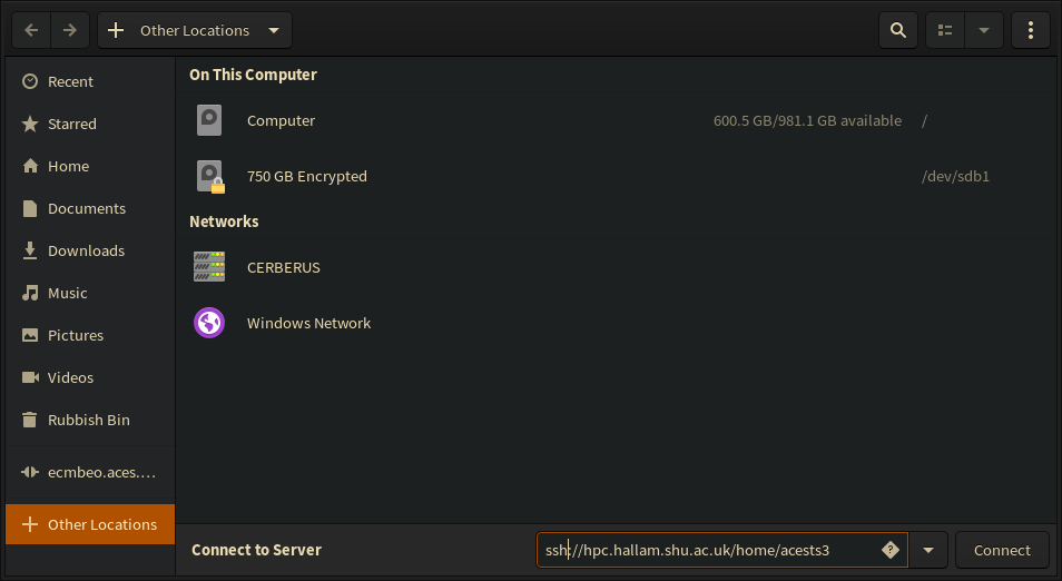
On a full Ubuntu (GNOME) installation you can simply use the file manager to attach the cluster file system, by going to “Other Locations” and entering the ssh:// URL for your cluster (don’t forget the username!). You should also add /home/USERNAME so you connect to your own home directory (if you forget that you’ll end in the “root” / of the file system and need to navigate to your home directory manually). You can bookmark this for easy access.
8.4.1.2. Windows/Mac (and Linux, but no need to in most cases):
FileZilla is a very capable File Transfer Protocol (FTP) client that is available for all platforms, so you can use it on Windows and Mac - also on Linux, if you do not like the shell commands and the native integration in the file manager is not enough:
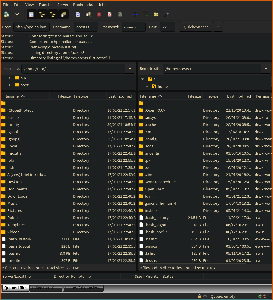
You will need to use port 22!
8.4.2. The better way:
For those of you who have embraced the command line more fully, there are, of course, several command line tools to copy files between machines. The most powerful is the command rsync. It has many options so you may want to look at the documentation man rsync. Many of the options won’t make sense at first, and we will only use a few. The simplest is copying a case directory to the cluster:
~/OpenFOAM/acests3-7/run
❯ rsync -avp HT-FSI3 acests3@hpc.hallam.shu.ac.uk:OpenFOAM/acests3-7/run/
sending incremental file list
HT-FSI3/
HT-FSI3/Allclean
HT-FSI3/Allrun
HT-FSI3/HT-FSI3.foam
HT-FSI3/PyFoamHistory
HT-FSI3/0/
HT-FSI3/0/fluid/
HT-FSI3/0/fluid/U
HT-FSI3/0/fluid/p
HT-FSI3/0/fluid/pointMotionU
HT-FSI3/0/solid/
HT-FSI3/0/solid/D
HT-FSI3/0/solid/DD
HT-FSI3/0/solid/pointD
HT-FSI3/0/solid/pointDD
HT-FSI3/constant/
HT-FSI3/constant/fsiProperties
HT-FSI3/constant/physicsProperties
HT-FSI3/constant/fluid/
HT-FSI3/constant/fluid/dynamicMeshDict
HT-FSI3/constant/fluid/fluidProperties
HT-FSI3/constant/fluid/transportProperties
HT-FSI3/constant/fluid/polyMesh/
HT-FSI3/constant/fluid/polyMesh/blockMeshDict
HT-FSI3/constant/fluid/polyMesh/blockMeshDict.first
HT-FSI3/constant/fluid/polyMesh/boundary
HT-FSI3/constant/fluid/polyMesh/faces
HT-FSI3/constant/fluid/polyMesh/neighbour
HT-FSI3/constant/fluid/polyMesh/owner
HT-FSI3/constant/fluid/polyMesh/points
HT-FSI3/constant/solid/
HT-FSI3/constant/solid/dynamicMeshDict
HT-FSI3/constant/solid/g
HT-FSI3/constant/solid/mechanicalProperties
HT-FSI3/constant/solid/solidProperties
HT-FSI3/constant/solid/polyMesh/
HT-FSI3/constant/solid/polyMesh/blockMeshDict
HT-FSI3/constant/solid/polyMesh/boundary
HT-FSI3/constant/solid/polyMesh/faces
HT-FSI3/constant/solid/polyMesh/neighbour
HT-FSI3/constant/solid/polyMesh/owner
HT-FSI3/constant/solid/polyMesh/points
HT-FSI3/history/
HT-FSI3/history/0/
HT-FSI3/history/0/solidPointDisplacement_pointDisp.dat
HT-FSI3/system/
HT-FSI3/system/controlDict
HT-FSI3/system/decomposeParDict
HT-FSI3/system/fluid/
HT-FSI3/system/fluid/decomposeParDict
HT-FSI3/system/fluid/fvSchemes
HT-FSI3/system/fluid/fvSolution
HT-FSI3/system/solid/
HT-FSI3/system/solid/controlDict
HT-FSI3/system/solid/decomposeParDict
HT-FSI3/system/solid/fvSchemes
HT-FSI3/system/solid/fvSolution

sent 1,109,151 bytes  received 996 bytes  444,058.80 bytes/sec
total size is 1,105,750  speedup is 1.00

~/OpenFOAM/acests3-7/run
❯
Use an uppercase P instead of the lower case p if you want the [P]rogress to show with more detail (like transfer speeds).
rsync is very economic, since it will only copy files that have changed on the source, so if you only have edited a boundary condition since the last rsync, it will only copy that one file over.
The basic syntax is like cp, so rsync -avp SOURCE TARGET, where both SOURCE and TARGET can be remote locations, which have the syntax USER@MACHINE:DIRECTORY, with DIRECTORY being relative to the user’s home directory, so if you want to copy to the home directory you end with the colon.
IMPORTANT: The / at the end is used when you want to copy into that directory, without it, you copy the source to be the target directory. So the command
rsync -avp HT-FSI3 acests3@hpc.hallam.shu.ac.uk:OpenFOAM/acests3-7/run/FSI3
would create a directory FSI3 on the remote machine, which will have the content of the source HT-FSI3 on the local machine.
TIP: If you have set up an ssh-key, then tab-completion will work for the remote machine’s file system as well!.
8.4.3. The elegant way (fuse, sshfs and autofs)
A very elegant and transparent way to work with files on the cluster (or on any other unix based computer) is to mount the filesystem directly. Together with an automated mounting system, this makes it as convenient as if the files were stored locally.
This will work on a full Ubuntu install, but should also work on a WSL install (not tested, please let me know if you try this.)
Linux does not have drive letters, but different drives get mounted into the directory tree. E.g. the home directory is often on a separate drive to the system files, but this will not be obvious to the user, because in Unix systems /home simply becomes part of the directory tree, so it doesn’t matter to the user, where that filesystem is located physically.
Using three tools, fuse, autofs, and sshfs, we can configure a Linux system such that it will automatically mount the remote drives, when we access them.
8.4.3.1. Install the required packages
sudo apt install sshfs autofs
sudo modprobe fuse
usermod -a -G fuse <YOURUSERNAME>
The last command may not be necessary if your user is an admin user, but it can’t hurt.
8.4.3.2. Configuring ssh and autofs
First we need to create a set of ssh-keys for root, so we don’t have provide a password every time the connection is established (see above, but you have to do it as root):
❯ sudo -s
[sudo] password for acests3:

TS-ZBook-17-G2# ssh-keygen
Generating public/private rsa key pair.
Enter file in which to save the key (/root/.ssh/id_rsa):
Created directory '/root/.ssh'.
Enter passphrase (empty for no passphrase):
Enter same passphrase again:
Your identification has been saved in /root/.ssh/id_rsa
Your public key has been saved in /root/.ssh/id_rsa.pub
The key fingerprint is:
SHA256:ZVkBfLgi+VDfnTvqZvK+xKLxYMJCAEExnfKQZNnhHDc root@TS-ZBook-17-G2
The key's randomart image is:
+---[RSA 3072]----+
|=B*ooE   ..oo.   |
|.*++o . . oo.    |
|  =o   o .++ . . |
|   o  + .oo . o  |
|    .  +S.     . |
|   . .  .  .  o  |
|    . o + . o. . |
|     . o =.o+    |
|        . .B=.   |
+----[SHA256]-----+

TS-ZBook-17-G2# ssh-copy-id acests3@hpc.hallam.shu.ac.uk
/usr/bin/ssh-copy-id: INFO: Source of key(s) to be installed: "/root/.ssh/id_rsa.pub"
The authenticity of host 'hpc.hallam.shu.ac.uk (10.14.120.60)' can't be established.
ECDSA key fingerprint is SHA256:SAV3T1nyQSwdh2Qzijod/4E333gNuqrsmdKxMDOiKSg.
Are you sure you want to continue connecting (yes/no/[fingerprint])? yes
/usr/bin/ssh-copy-id: INFO: attempting to log in with the new key(s), to filter out any that are already installed
/usr/bin/ssh-copy-id: INFO: 1 key(s) remain to be installed -- if you are prompted now it is to install the new keys
acests3@hpc.hallam.shu.ac.uk's password:

Number of key(s) added: 1

Now try logging into the machine, with:   "ssh 'acests3@hpc.hallam.shu.ac.uk'"
and check to make sure that only the key(s) you wanted were added.

TS-ZBook-17-G2#
We need to create a folder where the remote folder should be mounted.
sudo mkdir /mnt/sshfs
We need to know the userid (if you are the only user on a Ubuntu system, this most likely is going to be 1000, but it’s best to check):
user@machine:~$cat /etc/passwd | grep <YOURUSERNAME>
<YOURUSERNAME>:x:1000:1000:<Your Name>,,,:/home/<YOURUSERNAME>:/bin/bash
So the userid is 1000. So we add the following line to /etc/auto.master (you will need to use sudo and your favourite text editor for this, e.g. sudo nano /etc/auto.master, because /etc contains system configuration files that are only editable by the super-user):
/mnt/sshfs /etc/auto.sshfs uid=1000,gid=1000,--timeout=30,--ghost
and finally we need to create the file /etc/auto.sshfs and add a line like this:
hpc -fstype=fuse,rw,nodev,nonempty,noatime,allow_other,max_read=65536, reconnect,ServerAliveInterval=15,ServerAliveCountMax=3 :sshfs\#<YOURUSERNAME>@hpc.hallam.shu.ac.uk\:
This will mount the remote system in the folder mnt/sshfs/hpc every time we access that folder. If you are not using the folder for 30 seconds it will be unmounted.
Final words If you have several servers you just need to add line for each in the file /etc/auto.sshfs. Finally it should also be stated that the are some security considerations to take into account. If this done on a laptop and the laptop is stolen the burglar could gain access to the remote systems.
8.5. Running cases on the cluster
8.5.1. Case preparation
All cases have to be prepared to run as a batch process (without user interaction). Descriptions in this document are mostly for OpenFOAM, refer to the documentation of your code for instructions how to prepare cases for batch processing.
OpenFOAM cases will be ready to run in batch mode without any special measures. The only thing you should do is prepare them for parallel runs, i.e. run decomposePar (this can be done on the cluster, or on the pre-processing machine).
8.5.2. Scheduler
The cluster runs the SLURM workload manager. All cases have to be run through this. No interactive runs are allowed on the cluster.
When you log into the cluster, you will be on a login node. This is the only node that will allow you to use an interactive session directly. For everything else you need to ask SLURM to allocate resources to you. Resources are
- CPU/GPU
- memory
- time
I will only explain the basics here, please refer to the SLURM documentation for more.
8.5.2.1. Basic Slurm commands:
sinfo: gives you information on the cluster and if there are any free nodes
[acests3@ecmbeo1 ~]$ sinfo
PARTITION AVAIL  TIMELIMIT  NODES  STATE NODELIST
normal*      up 1-00:00:00      1  down* ecmbeo6
normal*      up 1-00:00:00      1  alloc ecmbeo5
normal*      up 1-00:00:00      4   idle ecmbeo[1-4]
long         up   infinite      1  down* ecmbeo6
long         up   infinite      1  alloc ecmbeo5
long         up   infinite      4   idle ecmbeo[1-4]
[acests3@ecmbeo1 ~]$
This tells you, that ecmbeo has 6 nodes, 5 of which are running, 1 is allocated (running a job), 4 are idle (available). One node (ecmbeo6) is not running and is down.
squeue: shows the queue, with all running and all waiting jobs
[acests3@ecmbeo1 ~]$ squeue
             JOBID PARTITION     NAME     USER ST       TIME  NODES NODELIST(REASON)
              1001    normal      HT3  acests3  R       01:12:04      1 ecmbeo5
[acests3@ecmbeo1 ~]$
So there is one job on ecmbeo5, in the normal partition (queue) 14, with name HT3, run by user acests3, in state (ST) [R]unning, for 1 hour, 12 minutes, and 4 seconds, using a single (1) node.
sbatch: sends cases to the queue to be run on the cluster.
The general syntax is:
sbatch -n <number of cores> -N <number of nodes> -p <partition/queue> <batch_script>
Some examples:
sbatch -n 8 run_script.sh
is the simplest sbatch command. It sends the run_script.sh to be executed on 8 cores.
sbatch -n 16 -p long run_script.sh
uses 16 cores and asks for the long partition, so the job will run longer than 24h on ecmbeo 15.
sbatch -n 24 -N 1 run_script.sh
sends the job to run on 24 cores and requests those 24 cores to be on a single node. This may be required if the job doesn’t work well on distributed memory (between nodes).
8.5.2.2. Job run scripts for SLURM
For most cases, Slurm requires a script that runs the command with the right settings. A script for OpenFOAM version 1912 will look like this 16:
#!/bin/bash

# The name of the script is FOAM
#SBATCH -J FOAM
# errors are written to:
#SBATCH -e error_file.e
# default output file (overridden with log file below)
#SBATCH -o output_file.o

# load mpi module (on hpc.hallam)
# comment this out on ecmbeo:
module load openmpi/gcc/64/1.10.1

# Initialises OpenFOAM (adjust according to your version)
source /home/acests3/OpenFOAM/OpenFOAM-v1912/etc/bashrc
# source /home/acests3/OpenFOAM/OpenFOAM-7/etc/bashrc
# source /opt/OpenFOAM/OpenFOAM-v1912/etc/bashrc
# source /opt/OpenFOAM/OpenFOAM-7/etc/bashrc


# Set foam application (adjust to fit your case):
export foamApp="pimpleFoam"
# Use directory that the sbatch is submitted from as case directory
# (start cases from case directory!)
export foamCase=`pwd`

# Start foam using mpirun
mpirun -np $SLURM_NPROCS $foamApp -case $foamCase -parallel > FOAM_$SLURM_JOB_ID.log
IMPORTANT: On hpc.hallam you will use my installation of OpenFOAM, which is in /home/acests3/OpenFOAM/ so do not change the home directory to your own one, unless you have your own installation of OpenFOAM.
You can find a template script in my home directory and copy it from there. The file needs to go into the case directory on the cluster.
cp ~acests3/run_foam.sh ./
Footnotes:
Although I have not ever lost a Windows installation this way, make a backup. I will not be responsible if you loose data!
LTS versions of Ubuntu are Long Term Support versions, intended for professional or corporate use. They release in a 2 year cycle. So they are a safe bet, if you prioritise stability over new features. You can also install the lastest release, but note that some software only releases packages for LTS releases.
WARNING: Since MS decided to use virtualisation for WSL2 activating WSL2 will not allow the use of other virtualisation layers, like VMWare or VirtualBox, Docker containers may also behave strangely. I do not have a Windows system to test this.
You can install several versions of OpenFOAM at the same time. You will decide which one to use when you initialise OpenFOAM. I have about 6 different versions installed at the moment.
solids4Foam is an alternative Fluid-Structure-Interaction framework, implemented in OpenFOAM alone (both solid and fluid solvers).
Note that the current version is version 9, but solids4Foam is not tested with that.
Don’t go on Reddit and ask that question, unless you want to start a religious war. Although that’s already going on, so you may as well… bring popcorn…
I now use Pop-OS, which is a derivative of Ubuntu, but has a slighlty different user interface philosophy.
Tip: Press the Super or Windows key to get the application launcher.
… is the title of a great book by Neal Stephenson.
… even on Windows, where every MS help article I need, starts with the words “launch Powershell as administrator”
I recommend notepad++
In incompressible flow, the actual pressure is not needed. It is, therefore, common to use only relative pressures in simulations.
Windkessel BCs were implemented using code developed by Andris Piebalgs at Imperial College Piebalgs2017,Piebalgs2018,Pirola2017.
The BCs are set in the boundary condition/time directory 0 in two files:
- the
pboundary condition file, where each WK outlet gets an entry of the form
ecmbeo has two partitions: normal and long. normal jobs are limited to 24h. long jobs are unlimited. You have to ask for the long queue explicitely. hpc.hallam does not have a runtime limit.
not needed on hpc.hallam where all jobs are unlimited.
adapt for OF7 and fe40, or to run on ecmbeo