Windkessel Python Module

1. Derivation of windkessel equations
2. Python module
- 2.1. Windkessel Models
  - 2.1.1. TODO reformulate without $\frac{d^{2}I}{dt^{2}}$
- 2.2. Waveform Approximation
3. Using the module
4. Validation of 3- and 4-element windkessel models
5. Parameter optimisation
- 5.1. Monte Carlo Method
  - 5.1.1. TODO Run local minimum scan
  - 5.1.2. TODO 4/5 element windkessel optimisation
- 5.2. Nelder-Mead Optimisation
  - 5.2.1. Comparison of 3-, 4-, and 5-element windkessel models with Nelder-Mead optimised parameters. ATTACH
6. Bibliography

1 Derivation of windkessel equations

$R_{c}$: characteristic impedance
$R_{p}$: peripheral resistance
$C$: compliance/capacitance
$L$: inductance

1.1 2-Element Windkessel model (wk2)

\[ \frac{dP(t)}{dt} = \frac{1}{C} I(t) - \frac{P(t)}{C R_{p}} \]

1.2 3-Element Windkessel model (wk3) and 4-element Windkessel model with serial impedance (wk4s)

\[ \frac{dP(t)}{dt} = \frac{1}{C} \left(1+\frac{R_{c}}{R_{p}}\right)I(t) + R_{c} \frac{dI(t)}{dt} - \frac{P(t)}{C R_{p}dt} = \frac{1}{C} \left(1+\frac{R_{c}}{R_{p}}\right)I(t) + R_{c} \frac{dI(t)}{dt} - \frac{P(t)}{C R_{c}} + \frac{L}{R_{p}C} \frac{dI(t)}{dt} + L \frac{d^{2}I(t)}{dt^{2}} \]

1.2.1 Alternative implementation in $P_{2}$ without $\frac{d^{2}I}{dt^{2}}$

If we express the model in terms of $P_{2}$, then the ODE for the 2-element windkessel model applies for the downstream part after $R_{c}$ and $L$:

\[ \frac{dP_{2}(t)}{dt} = \frac{1}{C} I(t) - \frac{P_{2}(t)}{C R_{p}} \]

For the 3- and 4-element windkessel with serial $L$, the pressure $P_{1}$ can then be expressed in terms of $P_{2}$ with an algebraic equation:

\[ P_{1}(t) = P_{2}(t) + R_{c} I(t) + L \frac{d I(t)}{dt} \]

Note: This implementation avoids the second derivative of I $\frac{d^{2}I}{dt}$ which can lead to numerical instabilities. This allows the use of lower order interpolations and approximations for the inlet waveform.

1.3 4-Element Windkessel model - parallel (wk4p)

\[ \frac{d^{2}P(t)}{dt^{2}} = R_{c} \frac{d^{2}I(t)}{dt^{2}} + \left( \frac{R_{c}}{R_{p} C} + \frac{1}{C} \right) \frac{dI(t)}{dt} + \frac{R_{c}}{C L} I(t) - \left( \frac{1}{R_{p} C} + \frac{R_{c}}{L} \right) \frac{dP(t)}{dt} + \frac{R_{c}}{R_{p} C L}P(t) \]

This is a second order ODE in p, which we need to reduce to a system of first order ODE, so the solve_ivp algorithm can integrate it. This is easily done by substituting a new variable for $d^{2}P / dt^{2}$:

\[ [dpdt] = \frac{dP}{dt} \]

\[ \frac{d[dpdt]}{dt} = R_{c} \frac{d^{2}I(t)}{dt^{2}} + \left( \frac{R_{c}}{R_{p} C} + \frac{1}{C} \right) \frac{dI(t)}{dt} + \frac{R_{c}}{C L} I(t) - \left( \frac{1}{R_{p} C} + \frac{R_{c}}{L} \right) [dpdt] + \frac{R_{c}}{R_{p} C L}P(t) \]

This system of coupled first order ODEs in p can be solved with solve_ivp.

Note: The system is still second order in $I$, but since $I$ is going to be given, we can calculate $\frac{dI}{dt}$ and $\frac{d^{2}I}{dt^{2}}$ using finite differences (see implementation below).

1.4 5-Element Windkessel model - parallel and serial inductance (wk5)

/Note: Also an alternative implementation of wk4p in $P_{2}$ without $\frac{d^{2}I}{dt^{2}}$

To avoid the second derivative in $I$, we can express the windkessel model in two ODEs in $p_{1}$, and $p_{2}$, similar to the wk3/wk4s-model above.

If both parallel and serial inductance are present in the model, then we can define this as a 5-element windkessel model (wk5). This model reduces to the 4-element windkessel model with parallel inductance (wk4p) if the serial inductance is set to zero.

\[ \frac{d p_{1}}{d t} = - \frac{R_{c}}{L_{p}} p_{1} + \left( \frac{R_{c}}{L_{p}} - \frac{1}{R_{p} C} \right) p_{2} + R_{c} \left( 1 + \frac{L_{s}}{L_{p}} \right) \frac{d I(t)}{d t} + \frac{I(t)}{C} \]

\[ \frac{d p_{2}}{d t} = - \frac{1}{R_{p} C} p_{2} + \frac{I(t)}{C} \]

In practice we then only need two implementations of the windkessel model, with or without parallel inductor:

wk: 4-element windkessel model with serial inductance that includes wk3 and wk2.
wk5: 5-element windkessel model with parallel and serial inductance that includes wk4p.

Both of these are implemented in the form without $d^{2} I/dt^{2}$.

2 Python module

2.1 Windkessel Models

After developing the windkessel models in Windkessel Modelling, I have implemented the windkessel solver as a python module. This module is available on github as part of the PySeuille Package¹.

The python module windkessel.py contains:

a documentation string:

#!/usr/bin/env python3
# -*- coding: utf-8 -*-

# This file is created automatically from org-mode [[roam:Windkessel Python Module]]

"""
Module for 2, 3, and 4 Element Windkessel Models

Calculates pressures before - p[y] - and after R1 - p[1]

usage:

import windkessel as wp

solve_wk(fun, Rc, Rp, C, L, time_start, time_end, N, method, initial_cond, rtol)

where:

fun:                    function object - volume flow

R1, R2, C, L:           windkessel parameters
                        set L = 0 for 3-Element WK
                        set R1 = 0 for 2-Element WK

Units:  either use physiological units (ml/s, mmHg/ml/s, ...)
        or SI units (m^3, Pa/m^3/s, ...), the result will be in
        consistent units (mmHg, or Pa)


Optional:

time_start, time_end:   start and end time for integration
                        (float, default: 0, 10)

N:                      number of time steps for result
                        (integer, default: 10000)

method:                 integration method (string, default: "RK45")
                        see solve_ivp documentation for available methods

initial_cond:           initial conditions
                        (2 element list for serial wk              default: [0, 0])
                        (3 element list for parallel 4-element wk  default: [0, 0, 0])

rtol:                   relative tolerance (float, default 1e-6)

@author: Torsten Schenkel, 2021
@license: MIT License
"""

Load the required modules:

import numpy as np
import scipy as sp
import scipy.integrate

We need the first and second time derivatives of the input volume flow rate, so define these using central differences:

def ddt(fun, t, dt):
    # Central differencing method
    return (fun(t + dt) - fun(t - dt)) / (2 * dt)


def d2dt2(fun, t, dt): 
    # Central differencing method
    return (fun(t + dt) - 2 * fun(t) + fun(t - dt)) / (dt ** 2)

The windkessel equation for the 2-element, 3-element, and 4-element windkessel with serial $R_{c}$ and $L$ can be defined in a uniform way. The distinction between the models is done via the parameters:
- $L = 0.0$ collapses the serial 4-element WK-equation to the 3-element WK-equation
- $Rc = 0.0$ collapses the 3-element WK-equation to the 2-element WK-equation

def wk_old(t, y, I, Rc, Rp, C, L, dt):
    # The 4-Element WK with serial L
    # set L = 0 for 3EWK
    # set L = 0, Rc = 0 for 2EWK
    #
    # Pressure at inlet:

    p1 = y[0]
    p2 = y[1]

    dp1dt = (
        Rc * ddt(I, t, dt)
        + (1 + Rc / Rp) * I(t) / C
        - p1 / (Rp * C)
        + L / (Rp * C) * ddt(I, t, dt)
        + L * d2dt2(I, t, dt)
    )
    # Pressure after proximal resistance:
    dp2dt = -p1 / (Rp * C) + (1 + Rc / Rp) * I(t) / C + L / (Rp * C) * ddt(I, t, dt)

    return [dp1dt, dp2dt]

/Note: New implementation is expressed in $p_{2}$ and avoids use of $\frac{d^{2}I}{dt^{2}}$:

def wk(t, y, I, Rc, Rp, C, L, dt):
    # The 4-Element WK with serial L
    # set L = 0 for 3EWK
    # set L = 0, Rc = 0 for 2EWK
    #
    # Pressure at inlet:

    p1 = y[0]
    p2 = y[1]

    # Do not solve an ODE for p1!
    # This is calculated algebraically later!
    dp1dt = 0.0

    # Pressure after proximal resistance:
    dp2dt = I(t) / C - p2 / (C * Rp)

    return [dp1dt, dp2dt]

The windkessel equation for the 4-element windkessel with $R_{c}$ and $L$ in parallel is a second order ODE in $p$ which can be transformed into a system of 2 first order ODEs:

2.1.1 TODO reformulate without $\frac{d^{2}I}{dt^{2}}$

def wk4p(t, y, I, Rc, Rp, C, L, dt):
    # The 4-Element WK with parallel L - obsolete: use wk5!
    p1 = y[0]
    p2 = y[1]
    dp1dt = y[2]
    d2pdt2 = (
        Rc * d2dt2(I, t, dt)
        + (Rc / Rp + 1 / C) * ddt(I, t, dt)
        + Rc / (C * L) * I(t)
        - Rc / (Rp * C * L) * p1
        - (1 / (Rp * C) + Rc / L) * dp1dt
    )
    # Second pressure not implemented yet!
    dp2dt = 0

    return [dp1dt, dp2dt, d2pdt2]

The formulation of a 4/5-element windkessel (I. Halliday 2021) avoids the second order time derivative of I and allows for both serial and parallel Inductances.

Note: This may be the preferred way to express this model, since it avoids $\frac{d^{2}I}{dt^{2}}$, which softens the smoothness requirements of the inlet waveform.

def wk5(t, y, I, Rc, Rp, C, Lp, Ls, dt):
    # The 4/5-Element WK with parallel Lp and serial Ls
    # changed from Ian's serial inertance being Lp in the Matlab code!
    # d_WM4E(1)  = -R1/L*WM4E(1) + (R1/L - 1/R2/C )*WM4E(2) + R1*(1+Lp/L)*didt + i/C;
    # d_WM4E(2)  =               - 1/R2/C          *WM4E(2)                    + i/C;

    dp1dt = (
        -Rc / Lp * y[0]
        + (Rc / Lp - 1 / Rp / C) * y[1]
        + Rc * (1 + Ls / Lp) * ddt(I, t, dt)
        + I(t) / C
    )

    dp2dt = -1 / Rp / C * y[1] + I(t) / C

    return [dp1dt, dp2dt]

Finally, we define wrapper functions to call the solve_ivp solver. All parameters can be given as named parameters. fun, Rc, Rp, and C (and L for the parallel 4-element model) must be given. All other parameters are optional and will use pre-defined defaults if omitted.

def solve_wk(
    fun,
    Rc,
    Rp,
    C,
    L=0,
    time_start=0,
    time_end=10,
    N=10000,
    method="RK45",
    initial_cond=[0, 0],
    rtol=1e-6,
    dt=1e-5,
):

    result = sp.integrate.solve_ivp(
        lambda t, y: wk(t, y, fun, Rc, Rp, C, L, dt),
        (time_start, time_end),
        initial_cond,
        t_eval=np.linspace(time_start, time_end, N),
        method=method,
        rtol=rtol,
        vectorized=True,
    )

    # p1 is not calculated from an ODE, but algebraically as:
    result.y[0] = result.y[1] + L * ddt(fun, result.t, dt) + Rc * fun(result.t)

    return result


def solve_wk4p(
    fun,
    Rc,
    Rp,
    C,
    L,
    time_start=0,
    time_end=10,
    N=10000,
    method="RK45",
    initial_cond=[0, 0, 0],
    rtol=1e-6,
    dt=1e-5,
):

    return sp.integrate.solve_ivp(
        lambda t, y: wk4p(t, y, fun, Rc, Rp, C, L, dt),
        (time_start, time_end),
        initial_cond,
        t_eval=np.linspace(time_start, time_end, N),
        method=method,
        rtol=rtol,
        vectorized=True,
    )


def solve_wk5(
    fun,
    Rc,
    Rp,
    C,
    Lp,
    Ls=0,
    time_start=0,
    time_end=10,
    N=10000,
    method="RK45",
    initial_cond=[0, 0, 0],
    rtol=1e-6,
    dt=1e-5,
):

    return sp.integrate.solve_ivp(
        lambda t, y: wk5(t, y, fun, Rc, Rp, C, Lp, Ls, dt),
        (time_start, time_end),
        initial_cond,
        t_eval=np.linspace(time_start, time_end, N),
        method=method,
        rtol=rtol,
        vectorized=True,
    )

2.2 Waveform Approximation

Flow rate waveform are very often scanned very roughly from echo-Doppler data and need to be interpolated to finer time-intervals. Typical interpolation, even piecewise higher order splines, can lead to oscillations. Furthermore, the approximated waveform should be smooth in it’s second-order derivative.

One solution to this problem is a third-order Bezier curve approximation. While this will result in an approximation, rather than an interpolation, the deviation in this implementation should be within the typical measurement uncertainty, and the behaviour of the curve is numerically benign, as it avoids jerks in the flow rate.

The functions take the scanned data as an ndarray, where data[0] contains an array of monotonously increasing x values (time), and data[1] contains an array of the respective y values (volume flow rate), e.g.:

vel = np.zeros((2, 15))

vel[0] = [0.0, 2.0, 4.5, 7.0, 12.0, 14.5, 19.5, 27.0, 34.5, 42.0, 49.5, 54.5, 72.0, 107.0, 142.0]

vel[1] = [0.0, 46.88, 85.94, 100.78, 108.6, 115.63, 115.63, 103.91, 85.16, 64.06, 45.31, 7.8125, 0.0, 0.0, 0.0]

The module contains functions to find the nearest and the lower time index on the data:

def nearest_time_index(t_array, t):

    t = t % np.max(t_array)

    idx = (np.abs(t_array - t)).argmin()

    return idx


def low_time_index(t_array, t):

    t = t % np.max(t_array)

    idx = nearest_time_index(t_array, t)

    if t_array[idx] > t:
        idx = idx - 1

    return idx

The approximation of the Bezier curve is done locally using the relative time $t_{int}$ within the piecewise curve segment:

\[ t_{int} = \frac{t - t_{n}}{t_{n+1} - T{n}} \]

and approximates a third-order Bezier curve based on the values at indices $n-1, n, n+1, n+2$.

Note: The index $n+2$ needs to be rolled over to $n=0$ for the last segment, where the lower time index is $n-1$

The local_PWBezier function will return the approximated value at time $t$ (needed for windkessel function definitions):

def local_PWBezier(data, t):
    '''
    local approximation of values for piecewise cubic Bezier approximator
    '''

    t = t % np.max(data[0])

    n = low_time_index(data[0], t)

    # Extend arrays by 1 (roll-over) for n+2 index!
    # time = np.append[data[0], data[0][0]]
    # data[1] = np.append[data[1], data[1][0]]

    # relative time between the reference points:
    intime = (t - data[0][n]) / (data[0][n + 1] - data[0][n])

    b0 = 1.0 / 6.0 * (data[1][n - 1] + 4.0 * data[1][n] + data[1][n + 1])
    b1 = 1.0 / 3.0 * (2 * data[1][n] + data[1][n + 1])
    b2 = 1.0 / 3.0 * (data[1][n] + 2 * data[1][n + 1])
    # last term includes rollover to -1 for n + 2
    if n < len(data[0]) - 2:
        b3 = 1.0 / 6.0 * (data[1][n] + 4 * data[1][n + 1] + data[1][n + 2])
    else:
        b3 = 1.0 / 6.0 * (data[1][n] + 4 * data[1][n + 1] + data[1][0])

    # b0 = 1.0 / 6.0 * (data[1][n - 2] + 4.0 * data[1][n - 1] + data[1][n])
    # b1 = 1.0 / 3.0 * (2 * data[1][n - 1] + data[1][n])
    # b2 = 1.0 / 3.0 * (data[1][n - 1] + 2 * data[1][n])
    # b3 = 1.0 / 6.0 * (data[1][n - 1] + 4 * data[1][n] + data[1][n + 1])

    return (
        pow((1.0 - intime), 3.0) * b0
        + 3.0 * pow((1.0 - intime), 2.0) * intime * b1
        + 3.0 * (1.0 - intime) * pow(intime, 2.0) * b2
        + pow(intime, 3.0) * b3
    )

While the PWBezier function will also work when given a time array by denumerating time-arrays and building a value array from the local approximations (needed for plots). This is the one that should be used to define the functions, since it works when called with a single time and a time array.

def PWBezier(data, t):
    '''
    Piecewise cubic Bezier curve approximator
    '''

    # Check if t is a float, if yes, call local approximator,
    # if not denumerate time array and create array of local approximations
    if isinstance(t, float):
        return local_PWBezier(data, t)
    else:
        v = np.zeros(t.shape)
        for idx, time in np.ndenumerate(t):
            v[idx[0]] = local_PWBezier(data, time)
        return v

3 Using the module

To use this, put the module somewhere in your PYTHONPATH or in the same directory as the calling code and import it using:

import windkessel as wk

Then the windkessel solver can be called with:

pressure = wk.solveWK(I, R1, R2, C, L)

Where I is a function object describing the volume flow waveform at the inlet of the windkessel as a function of time t.

This inlet waveform can be given in arbitrary units, but the other parameters need to be consistent, and the output will be in a unit that relates to input and parameter units. Typical units for the inlet volume flow are:

physiological: $[\mathrm{ml\ s^{-1}}]$
SI units: $[\mathrm{m^3\ s^{-1}}]$

Parameters are:

R1, R2: proximal and distal resistances in either $[\mathrm{mm_{Hg}\ ml^{-1}\ s}]$ or $[\mathrm{Pa\ s\ m^{-3}}]$.
C: compliance in either $[\mathrm{ml\ mm_{Hg}^{-1}}]$ or $[\mathrm{m^{3}\ Pa^{-1}}]$.
L: total arterial inertance in either $[\mathrm{mm_{Hg}\ s^{2}\ ml^{-1}}]$ or $[\mathrm{Pa\ s^{2}\ m^{-3}}]$.

The output of the windkessel model will be a 1-dimensional ndarray with two pressures (assuming the result of wk.solve_WK has been written into pressure as above):

pressure.y[0]: the pressure at the inlet of the windkessel
pressure.y[1]: the pressure after the proximal resistance for 3 and 4 element windkessel models

The pressure that is calculated by the windkessel will be in either $[\mathrm{mm_{Hg}}]$, or $[\mathrm{Pa}]$, depending on the units of input and the parameters.

Note that parameters found in literature are mostly in the physiological system, while the CFD code haemoFoam will require parameters in SI units!

3.1 Importing all the necessary modules

Copy windkessel.py into your PYTHONPATH or into the working directory of your project. Then import the module as usual (I use the shorthand wk):

import windkessel as wk

We will also need numpy and matplotlib.pyplot (I use the usual shorthand namespaces for the import here) ²:

import numpy as np
import matplotlib.pyplot as plt

# Seaborn makes the plots look a bit more modern
import seaborn as sns

sns.set_theme()
sns.set(rc={"figure.dpi": 300, "savefig.dpi": 300})
sns.set_style("white")

3.2 Setting the input waveform

The input waveform needs to be defined as a function object that returns a value for the volume flow rate as a function of the parameter time

3.2.1 Generic sine based waveform with dicrotic notch

In this example I use a generic waveform that is based on a sine wave with a period time $T$, a systolic time $T_{syst}$, and a dicrotic notch time of $T_{dicr}$. The maximum and minumum flow rates are given as $I_{max}$ and $I_{min}$.

This waveform is similar to the flow into the aorta, if $I_{min}$ is set to zero and a dicrotic notch time is used
It can also be used as a generic waveform for an artery further down the tree with $T_{dicr} = 0$ and a set $I_{min}$.

\[ f(x)=\begin{cases} (I_{max} - I_{min}) \sin(\pi \frac{t^{\%}}{T_{syst}} ) + I_{min} &, (t^{\%}) \leq (T_{syst}+T_{dicr})\\ I_{min} &, (t^{\%}) > (T_{syst}+T_{dicr}) \end{cases} \]

where $t^{\%}$ is $t$ modulo $T$, i.e. the time in the current period, $0 \leq t^{\%} < 1$.

Setting the waveform parameters:

# Generic Input Waveform
# max volume flow in ml/s
max_i = 425

# min volume flow in m^3/s
min_i = 0.0

# Period time in s
T = 0.9

# Syst. Time in s
systTime = 2 / 5 * T

# Dicrotic notch time
dicrTime = 0.03

Define the waveform as a function.

Note: I use a Boolean condition to implement the piecewise function!

def I_generic(t):
    # implicit conditional using boolean multiplicator
    # sine waveform
    I = (
        (max_i - min_i) * np.sin(np.pi / systTime * (t % T))
        *(t % T < (systTime + dicrTime)) + min_i
    )

    return I

So let’s have a look at the waveforms:

Note: I am already calling the ddt and d2dt functions from the windkessel module. They are prefixed with their namespace wk.

Note 2: The d2dt function as it is implemented (central difference) is not defined at the beginning of the time range. So autoscale will not work and give you a flat line on a huge y-axis scale!

t = np.linspace(0, 2, 2000)

plt.plot(t, I_generic(t), label="$\dot{V}$")
plt.plot(t, 0.1 * wk.ddt(I_generic, t, 0.0001), label="$d\dot{V}/dt$")
# plt.plot(t, 0.01 * wk.d2dt2(I_generic, t, 0.0001), label="$d^{2}\dot{V}/dt^{2}$")
plt.xlabel("time [$\\mathrm{s}$]")
plt.ylabel(
    "$\dot{V}\ [\mathrm{\\frac{ml}{s}}],\
    \\frac{d\dot{V}}{dt}\ [10\ \mathrm{\\frac{ml}{s^{2}}}],\
    # \\frac{d^{2}\dot{V}}{dt^{2}}\ [100\  \mathrm{\\frac{ml}{s^{3}}}]$"
)
plt.xlim(0, 2)
plt.ylim(-600, 500)
plt.grid()
plt.legend(loc="lower center", ncol=3);

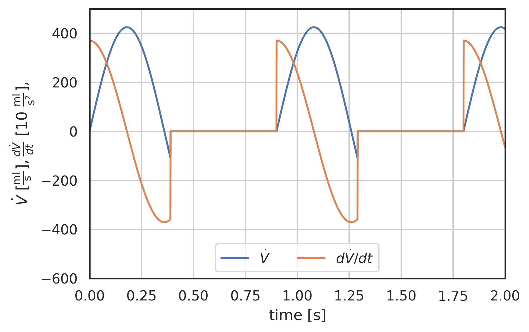
Figure 1: Generic sine based flow rate waveform, no dicrotic notch. And its first and second time-derivative

3.3 Solving the windkessel equations

The solution of the windkessel equations is then done using a simple command wk.solve_wk. The distinction between 2-element, 3-element, or 4-element windkessel models is done via selection of the model parameters Rc, Rp, C, and L. All parameters must be given, Rc and L can be set to 0.0 to eliminate the element from the model.

Note: Rp and C must not be set to zero, which would result in a division by zero.

Note 2: If C is set to a very low value the windkessel model may not finish successfully.

# Set parameters for 3-Element Windkessel Model
R1 = 0.03
R2 = 1
C = 2.0
Lp = 0.02

time_start = 0
time_end = 30
N = (time_end - time_start) * 1000

%time pressure3 = wk.solve_wk(I_generic, R1, R2, C, 0, time_start, time_end, N, "RK45", [0, 0], 1e-8)

%time pressure4 = wk.solve_wk5(I_generic, R1, R2, C, Lp, 0, time_start, time_end, N, "RK45", [0, 0], 1e-8)

# Note: all other parameters to wk.solve_wk are optional
#       if they are not given, defaults will be used
#       Here I use time range from 0 to 30 and 30000 steps
#       to override the default of 0, 10, 10000

And plot the result:

# the solution is returned as an array with labels 't' and 'y'
# where 'y' is a vector array with two entries
# y[0] - pressure before R1
# y[1] - pressure after R2

# plot curves
plt.xlabel("time [s]")
plt.ylabel("pressure [$\\mathrm{mm_{Hg}}$]")
plt.xlim(0, 30)

# plot first and second component (index 0, 1) of array 'y'
# over array 't':
plt.plot(pressure3.t, pressure3.y[0], label="$p_1, WK3$")
plt.plot(pressure3.t, pressure3.y[1], label="$p_2, WK3$")
plt.plot(pressure4.t, pressure4.y[0], label="$p_1, WK4$")
plt.plot(pressure4.t, pressure4.y[1], label="$p_2, WK4$")

plt.legend()
plt.grid()

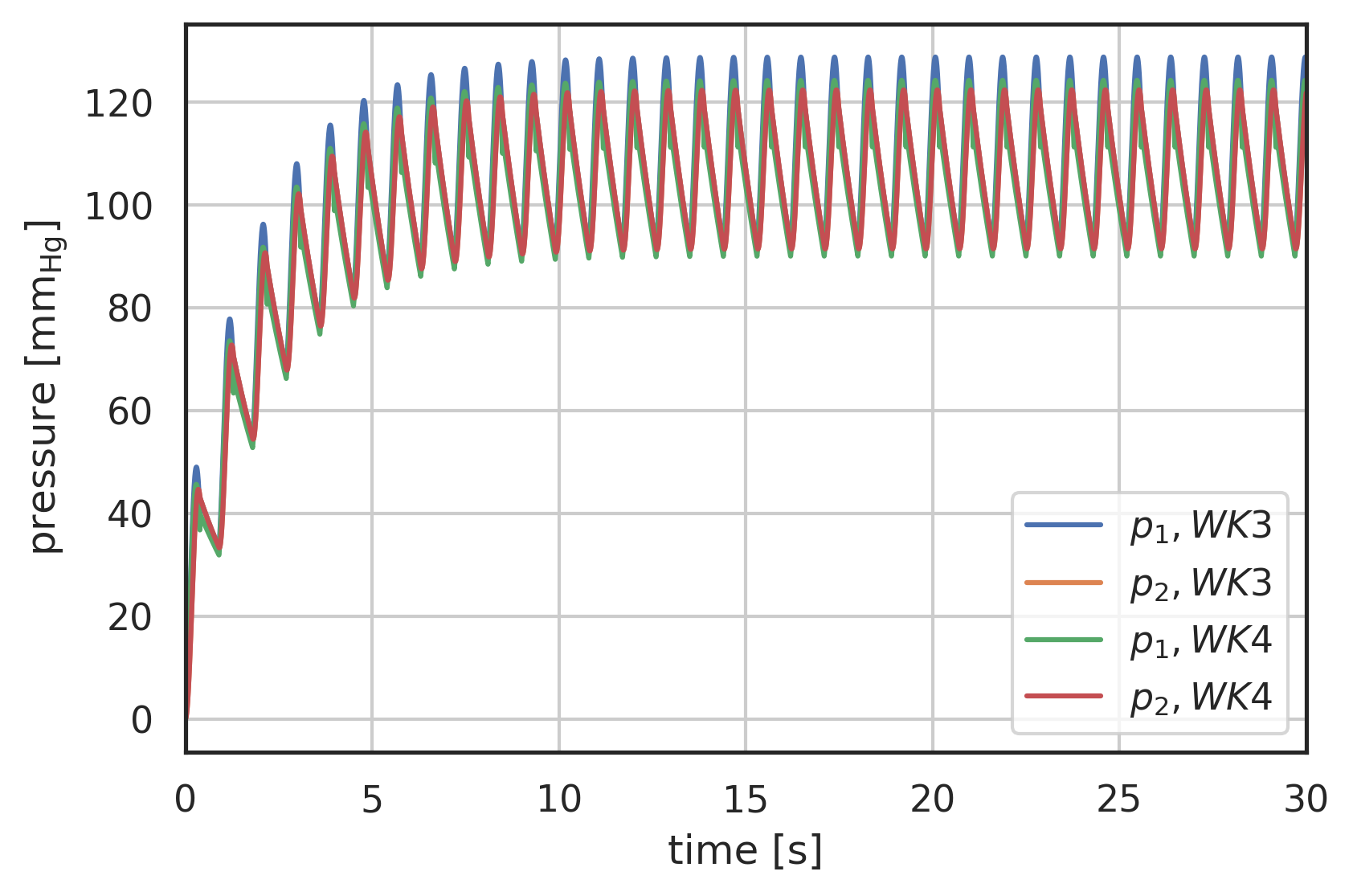
Figure 2: Pressure response to generic input waveform, 3-Element Windkessel model

Let’s have a closer look at the last 10% of that plot:

# plot curves
plt.xlabel("time [s]")
plt.ylabel("pressure [$\\mathrm{mm_{Hg}}$]")

startN = int(0.95 * N)
# plot first and second component (index 0, 1) of array 'y'
# over array 't':
plt.plot(pressure3.t[startN:], pressure3.y[0][startN:], label="$p_1, WK3$")
plt.plot(pressure3.t[startN:], pressure3.y[1][startN:], label="$p_2, WK3$")
plt.plot(pressure4.t[startN:], pressure4.y[0][startN:], label="$p_1, WK4$")
plt.plot(pressure4.t[startN:], pressure4.y[1][startN:], label="$p_2, WK4$")

plt.legend()
plt.grid()

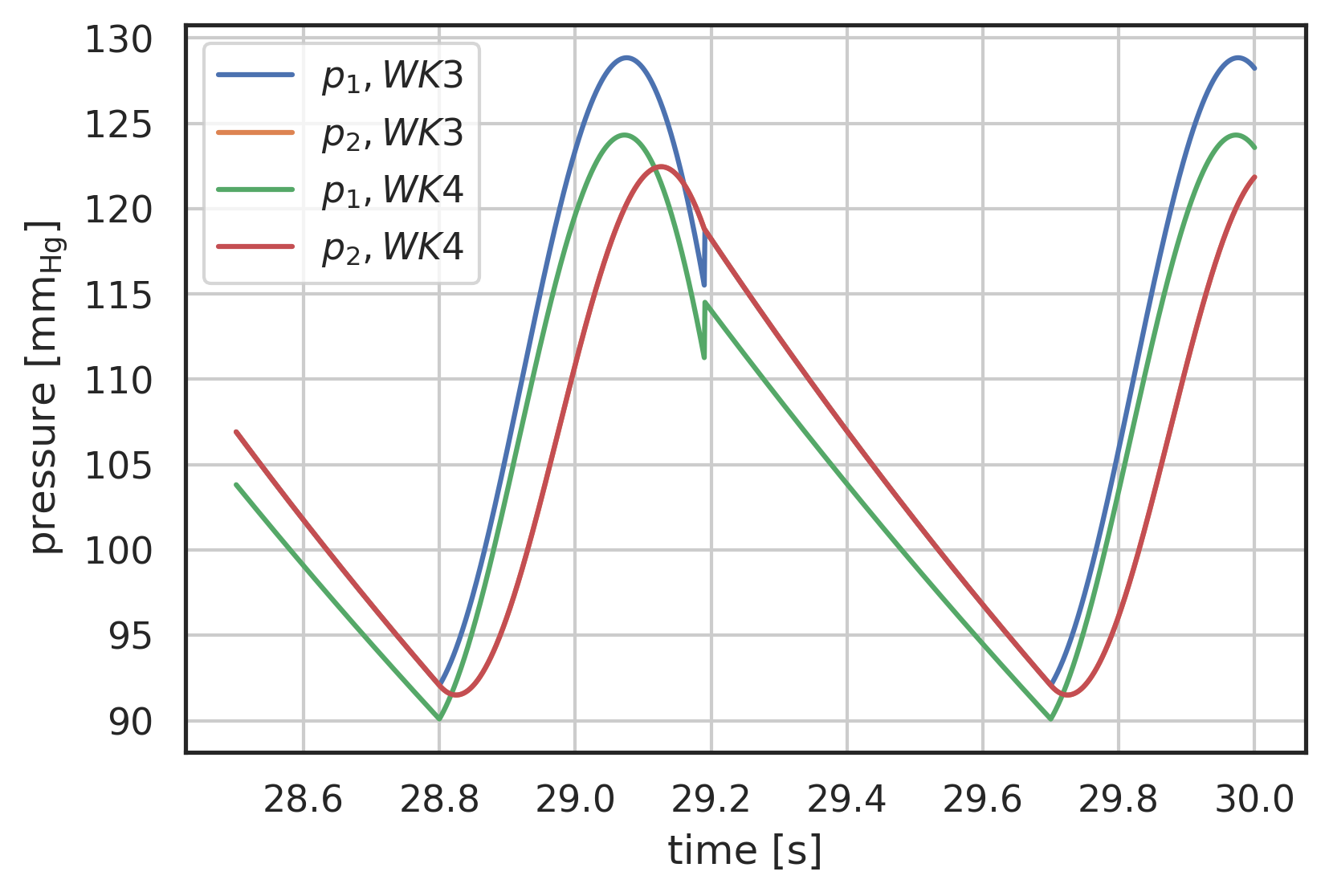
Figure 3: Pressure response to generic input waveform, 3-element and 4-element windkessel models, periodic state

3.4 Pedrizzetti waveform [Pedrizzetti1996]

# Parameters
C0 = 0.4355
C2 = 0.05
C4 = -0.13
C6 = -0.1
C8 = -0.01

S2 = 0.25
S4 = 0.13
S6 = -0.02
S8 = -0.03

# Area of the CCA
# area = 3e-5
area = 400


def I_ped(t):
    return (
        C0
        + C2 * np.cos(2 * np.pi * t)
        + S2 * np.sin(2 * np.pi * t)
        + C4 * np.cos(4 * np.pi * t)
        + S4 * np.sin(4 * np.pi * t)
        + C6 * np.cos(6 * np.pi * t)
        + S6 * np.sin(6 * np.pi * t)
        + C8 * np.cos(8 * np.pi * t)
        + S8 * np.sin(8 * np.pi * t)
    ) * area

t = np.linspace(0, 30, 30000)

plt.plot(t, I_ped(t), label="$\dot{V}$")
plt.plot(t, 0.1 * wk.ddt(I_ped, t, 1e-5), label="$d\dot{V}/dt$")
plt.plot(t, 0.01 * wk.d2dt2(I_ped, t, 1e-5), label="$d^{2}\dot{V}/dt^{2}$")
plt.xlabel("time [$\\mathrm{s}$]")
plt.ylabel(
    "$\dot{V}\ [\mathrm{\\frac{ml}{s}}],\
    \\frac{d\dot{V}}{dt}\ [10\ \mathrm{\\frac{ml}{s^{2}}}],\
    \\frac{d^{2}\dot{V}}{dt^{2}}\ [100\  \mathrm{\\frac{ml}{s^{3}}}]$"
)
plt.xlim(28, 30)
# plt.ylim(-600, 500)
plt.grid()
plt.legend(loc="lower center", ncol=3);

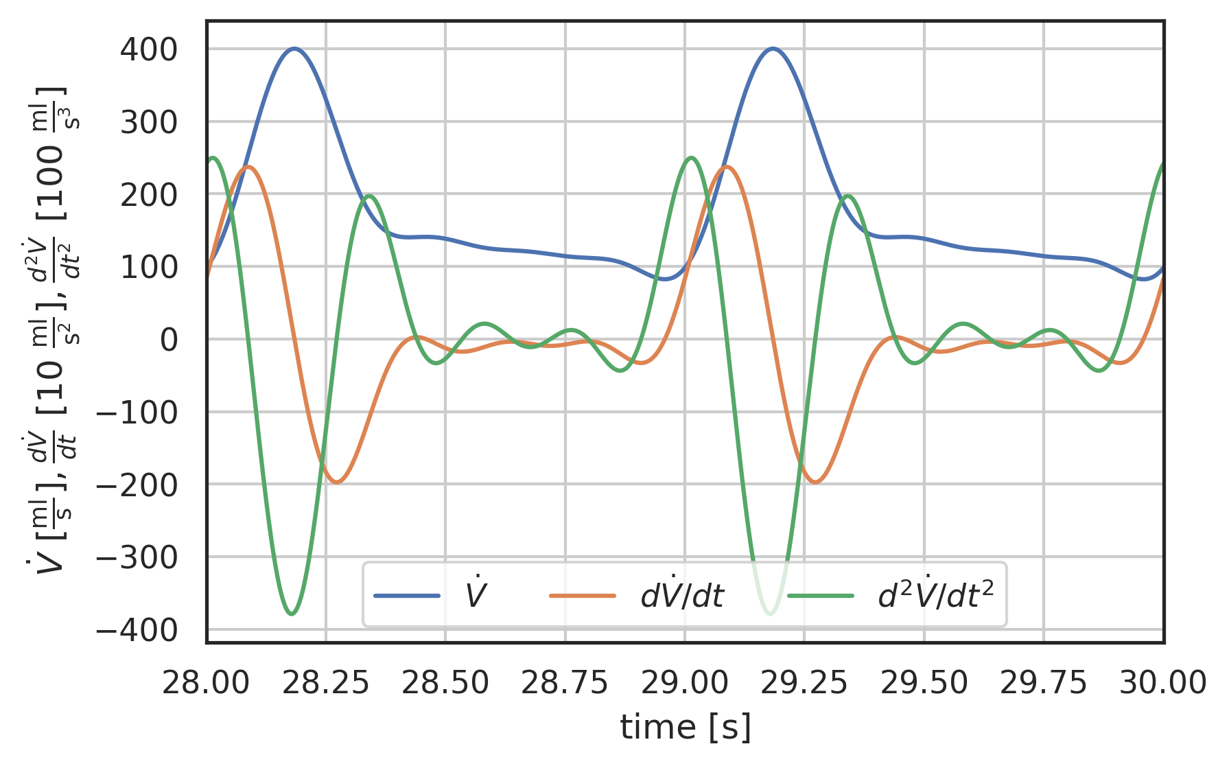
Figure 4: Physiological flow rate waveform, downstream from aorta, and its first and second time derivative

# Set parameters for Windkessel Model
Rc = 0.033
Rp = 0.6
C = 1.25
# L for serial model - pure serial will use 1/10 of this!
Ls = 0.02
# L for parallel
Lp = 0.02

time_start = 0
time_end = 30
N = (time_end - time_start) * 1000

fun = I_ped

pressure2wk = wk.solve_wk(
    fun=fun,
    Rc=0,
    Rp=Rp,
    C=C,
    L=0,
    time_start=0,
    time_end=30,
    N=30000,
    method="RK45",
    initial_cond=[0, 0],
    rtol=1e-9,
)

pressure3wk = wk.solve_wk(
    fun=fun,
    Rc=Rc,
    Rp=Rp,
    C=C,
    L=0,
    time_start=0,
    time_end=30,
    N=30000,
    method="RK45",
    initial_cond=[0, 0],
    rtol=1e-9,
)

pressure4wks = wk.solve_wk(
    fun=fun,
    Rc=Rc,
    Rp=Rp,
    C=C,
    L=Ls / 10,
    time_start=0,
    time_end=30,
    N=30000,
    method="RK45",
    initial_cond=[0, 0],
    rtol=1e-9,
)


pressure4wkp = wk.solve_wk4p(
    fun=fun,
    Rc=Rc,
    Rp=Rp,
    C=C,
    L=Lp,
    time_start=0,
    time_end=30,
    N=30000,
    method="RK45",
    initial_cond=[0, 0, 0],
    rtol=1e-9,
)

# Note: all other parameters to wk.solve_wk are optional
#       if they are not given, defaults will be used
#       Here I use time range from 0 to 30 and 30000 steps
#       to override the default of 0, 10, 10000

pressure5wk = wk.solve_wk5(
    fun=fun,
    Rc=Rc,
    Rp=Rp,
    C=C,
    Ls=Ls,
    Lp=Lp,
    time_start=0,
    time_end=30,
    N=30000,
    method="RK45",
    initial_cond=[0, 0],
    rtol=1e-9,
)

And plot the result:

# the solution is returned as an array with labels 't' and 'y'
# where 'y' is a vector array with two entries
# y[0] - pressure before R1
# y[1] - pressure after R2

# plot curves
plt.xlabel("time [s]")
plt.ylabel("pressure [$\\mathrm{mm_{Hg}}$]")
plt.xlim(0, 30)

# plot first and second component (index 0, 1) of array 'y'
# over array 't':
plt.plot(pressure2wk.t, pressure2wk.y[0], label="$p_1, WK2$")
plt.plot(pressure3wk.t, pressure3wk.y[0], label="$p_1, WK3$")
plt.plot(pressure4wks.t, pressure4wks.y[0], label="$p_1, WK4S$")
plt.plot(pressure4wkp.t, pressure4wkp.y[0], label="$p_1, WK4P$")
plt.plot(pressure5wk.t, pressure5wk.y[0], label="$p_1, WK5$")
# plt.plot(pressure.t, pressure.y[1], label="$p_2, WK4S$")
plt.legend()
plt.grid()

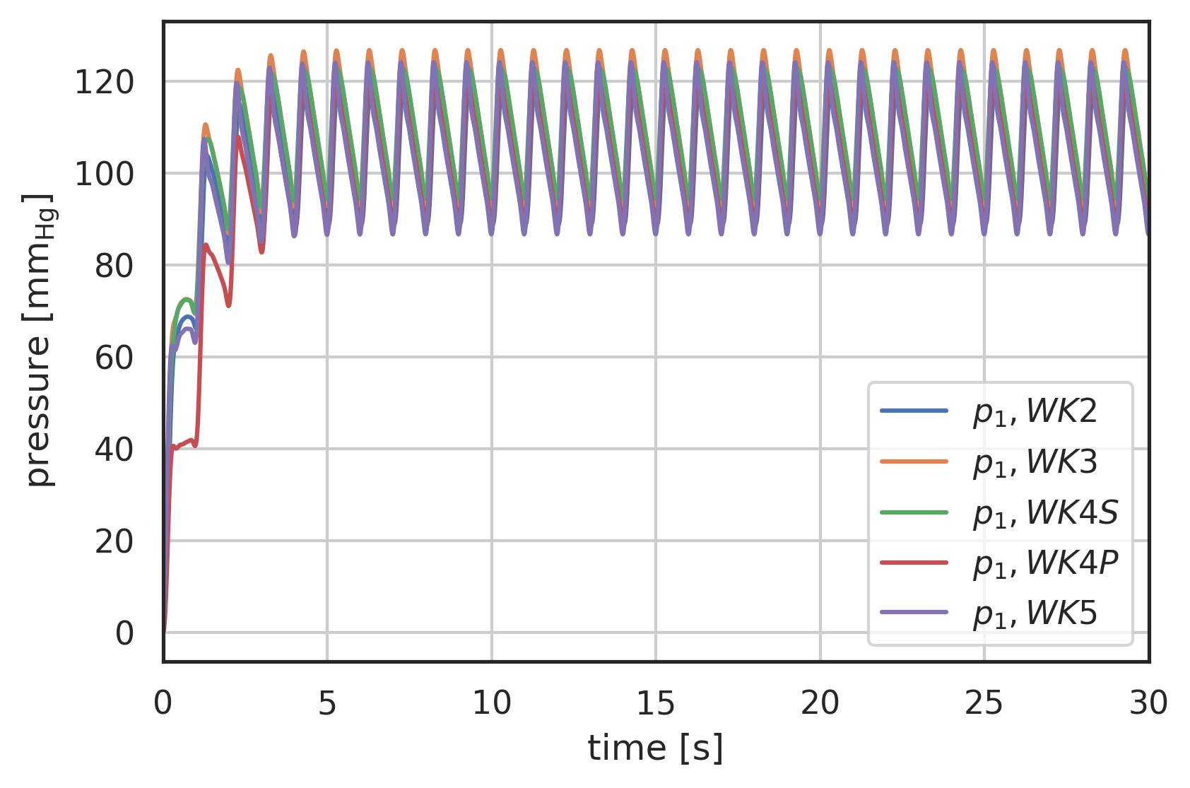
Figure 5: Pressure response to Pedrizzetti [Pedrizzetti1996] input waveform, comparison of 2-Element (WK2), 3-Element (WK3) and 4-Element Windkessel models (WK4S - serial, WK4P - parallel), development

# plot curves
plt.xlabel("time [s]")
plt.ylabel("pressure [$\\mathrm{mm_{Hg}}$]")

startN = int(0.9 * N)
# plot first and second component (index 0, 1) of array 'y'
# over array 't':
plt.plot(pressure2wk.t[startN:], pressure2wk.y[0][startN:], label="$p_1, WK2$")
plt.plot(pressure3wk.t[startN:], pressure3wk.y[0][startN:], label="$p_1, WK3$")
plt.plot(pressure4wks.t[startN:], pressure4wks.y[0][startN:], label="$p_1, WK4S$")
plt.plot(pressure4wkp.t[startN:], pressure4wkp.y[0][startN:], label="$p_1, WK4P$")
plt.plot(pressure5wk.t[startN:], pressure5wk.y[0][startN:], label="$p_1, WK5$")


# Plot the inlet waveform in lightgrey scaled to fit
t = np.linspace(28, 30, 2000)

scaledQ = (
    (I_ped(t) / np.max(I_ped(t))
    * (np.max(pressure3wk.y[0]) - np.min(pressure3wk.y[0][startN:]))
    + np.min(pressure3wk.y[0][startN:]))
)


plt.plot(t, scaledQ, color="lightgrey")

plt.xlim(28, 30)
plt.legend()
plt.grid()

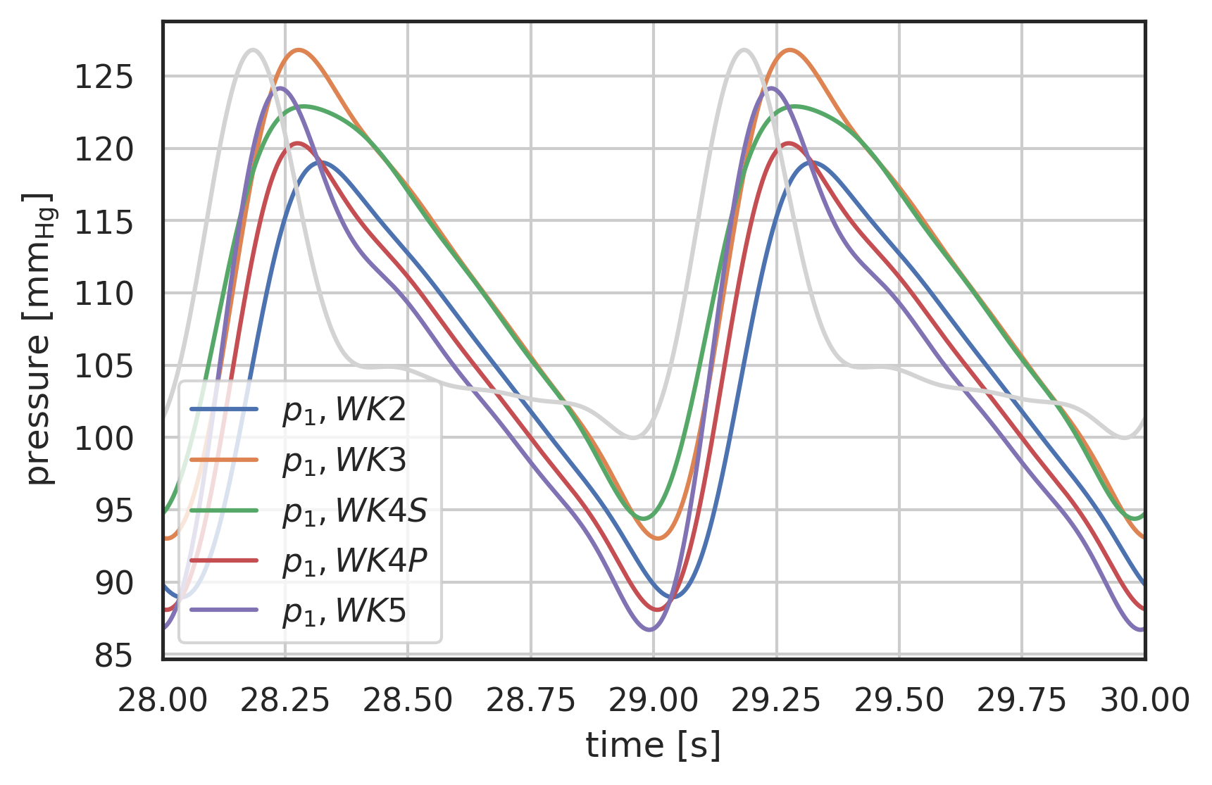
Figure 6: Pressure response to Pedrizzetti [Pedrizzetti1996] input waveform, comparison of 2-Element (WK2), 3-Element (WK3) and 4-Element Windkessel models (WK4S - serial, WK4P - parallel), periodic state

3.5 TODO Working with high temporal resolution volume flow data

If the volume flow data is measured with a high temporal resolution, the volume flow at any time can be obtained from

interpolation: scipy has many interpolation methods available. Most are unsuited to our case for two reasons:
- They are not second-order differentiable. The windkessel model is using the second time derivative of I. If the inlet waveform has jerks (2nd derivative discontinuities), then this can lead to numerical instabilities or non-physical results. While, e.g. Akima, or Pchip reproduce most measured waveforms very well, they are only first order differentiable.
- They are unbounded. Higher order interpolations, e.g. cubic splines, are second order differentiable, but can lead to unbounded oscillations, in particular for cases that show high frequency effects, e.g., dicrotic notch.
Fourier Transforms: FFT and IFFT are a good way to transform a discrete dataset into a continuous function that can be used for the windkessel model. However they require a high sampling rate to avoid oscillations (similar to higher order interpolations) and follow the original waveform closely.

3.5.1 TODO FFT/IFFT implementation

3.6 Working with low temporal resolution scanned volume flow data

In many cases the velocity is going to be measured using Echo-Doppler and needs to be scanned from the Echo images or is otherwise only available in a low time resolution. In this case we need to create a high time-resolution waveform from the low resolution data.

Interpolation leads to unbounded oscillations in this case, so we use a third order B-Spline approximation that will give a smooth second order differential.

Note: Since the B-Spline is bounded it will always stay on the concave side of the scanned data, i.e. bounded, but will not go through the measured points. The deviation is typically within the measurement uncertainty if the measurement is digitised with this in mind.

This method was developed for smooth 3-d B-Splines for 2nd order smooth prescribed movement of the ventricular wall and is described in [Schenkel2009]

Let’s test this using this rough waveform of an aortic flow, scanned from an Echo-Doppler printout. vol is a (2,15) array, where vol[0] is the time, and vol[1] the volume flow rate array.

vol = np.zeros((2, 15))

vol[0] = [0., 0.0125, 0.028125, 0.04375, 0.075, 0.090625, 0.121875, 0.16875, 0.215625, 0.2625, 0.309375, 0.340625, 0.45, 0.66875, 0.8875]
vol[1] = [0., 187.52, 343.76, 403.12, 434.4, 462.52, 462.52, 415.64, 340.64, 256.24, 181.24, -31.25, 0., 0., 0.]

plt.plot(vol[0], vol[1]);

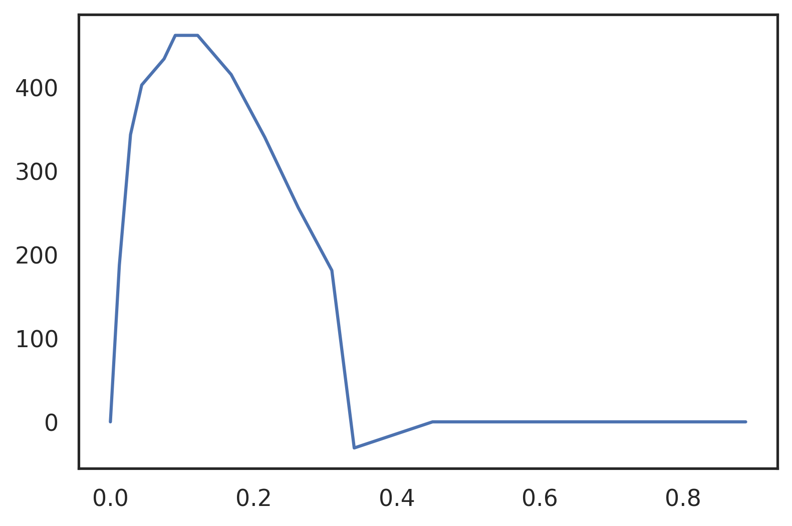
Figure 7: Coarsely sampled waveform of aortic flow. Only 16 sampling points over the whole cycle.

The approximated waveform function can be defined using wk.PWBezier

def I_Bezier(t):
    return wk.PWBezier(vol, t)

As we can show the approximated waveform follows the scanned waveform, but stays on the concave side and is bounded without any oscillations. It can be seen that the dicrotic notch is underrepresented. This shows that the resolution needs to be increased around that point.

Note: When digitising curves, make sure you include two points either side of a detail like this. These two points will define how far the approximation will be pulled into the notch.

ta = np.linspace(0, 2, 1000)
        
plt.plot(vol[0], vol[1], label='original')
plt.plot(ta, I_Bezier(ta), label='PWBezier')
plt.legend();

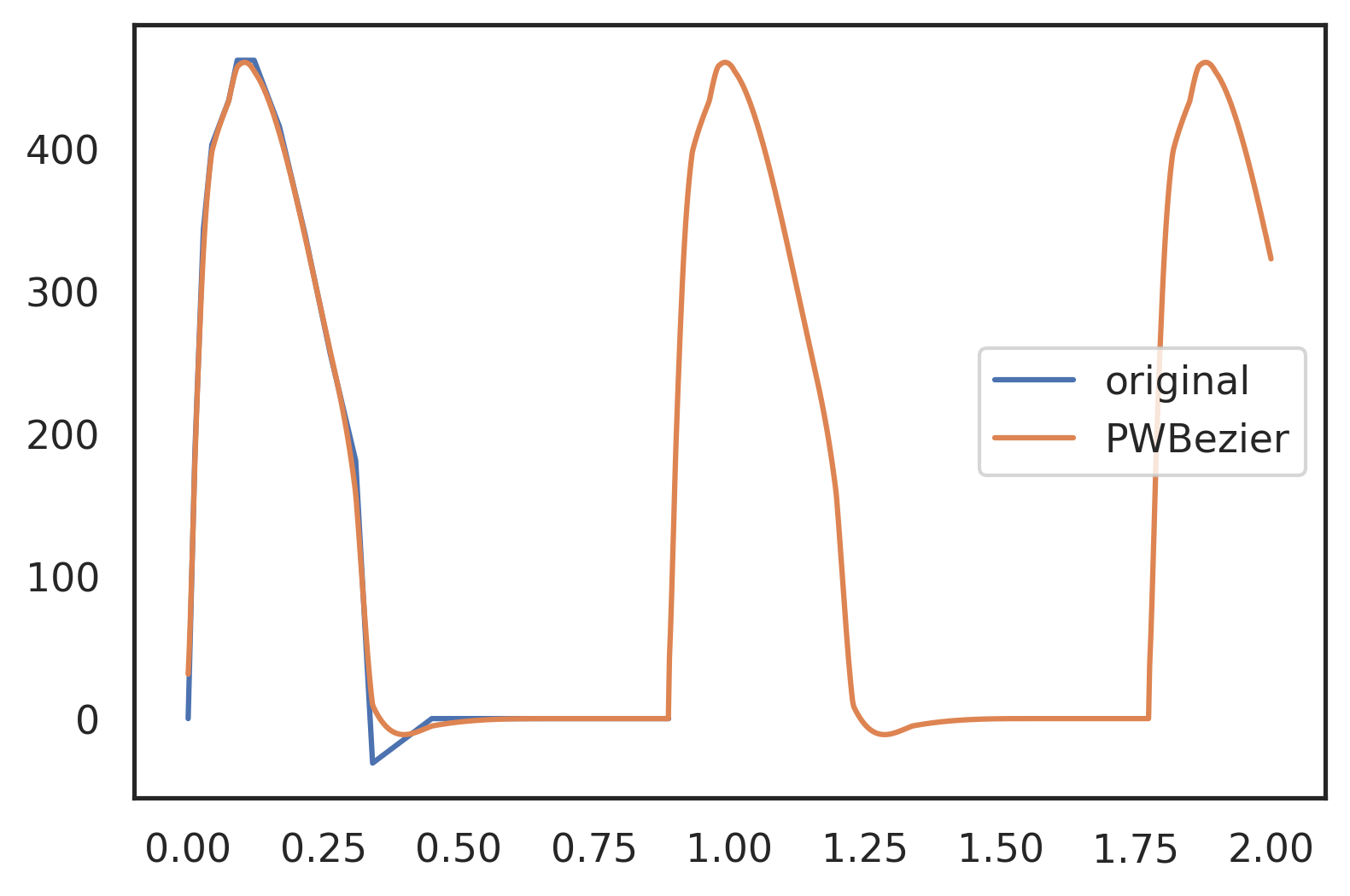
Figure 8: Piecewise B-Spline approximation of the coarse sample. The dicrotic notch is not represented to its original depth. This would need two additional points next to the single sampling point in the apex of the notch. Otherwise the approximation follows the original sample closely. Note that the approximation stays on the concave side.

# Set parameters for Windkessel Model
Rc = 0.03
Rp = 0.8
C = 2
# L for serial model - pure serial will use 1/10 of this!
Ls = 0.02
# L for parallel
Lp = 0.02

time_start = 0
time_end = 30
N = (time_end - time_start) * 1000

fun = I_Bezier

pressure2wk = wk.solve_wk(
    fun=fun,
    Rc=0,
    Rp=Rp,
    C=C,
    L=0,
    time_start=0,
    time_end=30,
    N=30000,
    method="RK45",
    initial_cond=[0, 0],
    rtol=1e-9,
)

pressure3wk = wk.solve_wk(
    fun=fun,
    Rc=Rc,
    Rp=Rp,
    C=C,
    L=0,
    time_start=0,
    time_end=30,
    N=30000,
    method="RK45",
    initial_cond=[0, 0],
    rtol=1e-9,
)

pressure4wks = wk.solve_wk(
    fun=fun,
    Rc=Rc,
    Rp=Rp,
    C=C,
    L=Ls/20.0,
    time_start=0,
    time_end=30,
    N=30000,
    method="RK45",
    initial_cond=[0, 0],
    rtol=1e-9,
    dt=1e-5
)


pressure4wkp = wk.solve_wk5(
    fun=fun,
    Rc=Rc,
    Rp=Rp,
    C=C,
    Ls=0.0,
    Lp=Lp,
    time_start=0,
    time_end=30,
    N=30000,
    method="RK45",
    initial_cond=[0, 0],
    rtol=1e-9,
)

# Note: all other parameters to wk.solve_wk are optional
#       if they are not given, defaults will be used
#       Here I use time range from 0 to 30 and 30000 steps
#       to override the default of 0, 10, 10000

pressure5wk = wk.solve_wk5(
    fun=fun,
    Rc=Rc,
    Rp=Rp,
    C=C,
    Ls=Ls,
    Lp=Lp,
    time_start=0,
    time_end=30,
    N=30000,
    method="RK45",
    initial_cond=[0, 0],
    rtol=1e-9,
)

And plot the result:

# the solution is returned as an array with labels 't' and 'y'
# where 'y' is a vector array with two entries
# y[0] - pressure before R1
# y[1] - pressure after R2

# plot curves
plt.xlabel("time [s]")
plt.ylabel("pressure [$\\mathrm{mm_{Hg}}$]")
plt.xlim(0, 30)

# plot first and second component (index 0, 1) of array 'y'
# over array 't':
plt.plot(pressure2wk.t, pressure2wk.y[0], label="$p_1, WK2$")
plt.plot(pressure3wk.t, pressure3wk.y[0], label="$p_1, WK3$")
plt.plot(pressure4wks.t, pressure4wks.y[0], label="$p_1, WK4S$")
plt.plot(pressure4wkp.t, pressure4wkp.y[0], label="$p_1, WK4P$")
plt.plot(pressure5wk.t, pressure5wk.y[0], label="$p_1, WK5$")
# plt.plot(pressure.t, pressure.y[1], label="$p_2, WK4S$")
plt.legend()
plt.grid()

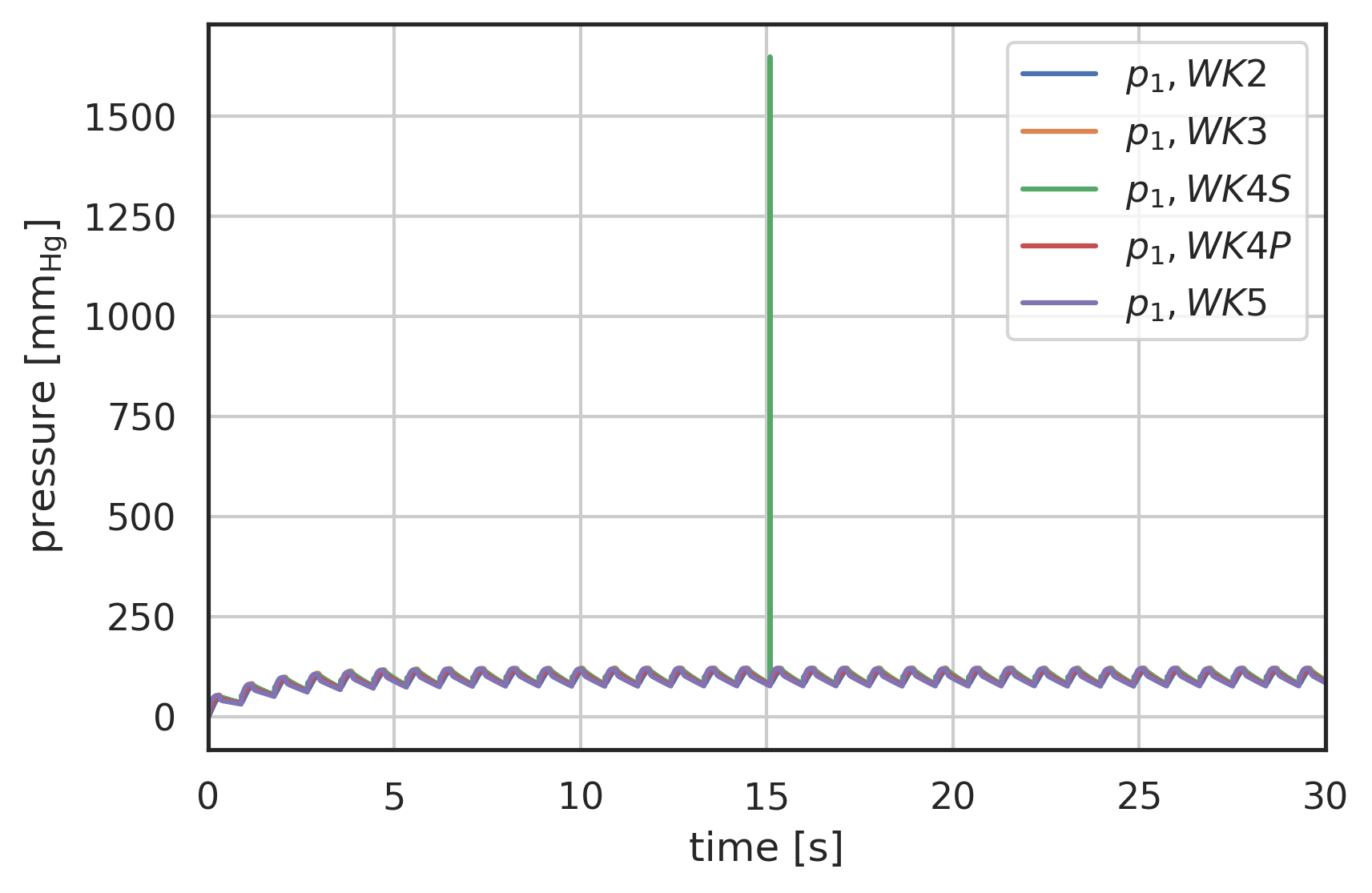
Figure 9: Pressure response to coarse scan input waveform, comparison of 2-Element (WK2), 3-Element (WK3) and 4-Element Windkessel models (WK4S - serial, WK4P - parallel), development

# plot curves
plt.xlabel("time [s]")
plt.ylabel("pressure [$\\mathrm{mm_{Hg}}$]")

startN = int(0.9 * N)
# plot first and second component (index 0, 1) of array 'y'
# over array 't':
plt.plot(pressure2wk.t[startN:], pressure2wk.y[0][startN:], label="$p_1, WK2$")
plt.plot(pressure3wk.t[startN:], pressure3wk.y[0][startN:], label="$p_1, WK3$")
plt.plot(pressure4wks.t[startN:], pressure4wks.y[0][startN:], label="$p_1, WK4S$")
plt.plot(pressure4wkp.t[startN:], pressure4wkp.y[0][startN:], label="$p_1, WK4P$")
plt.plot(pressure5wk.t[startN:], pressure5wk.y[0][startN:], label="$p_1, WK5$")
# plt.plot(
#     pressure.t[startN:],
#     pressure.y[0][startN:]
#     - R1 * I_generic(pressure.t[startN:])
#     - L * wk.ddt(I_generic, pressure.t[startN:]),
#     label="p_2 analytical",
# )

t = np.linspace(28, 30, 2000)
plt.plot(
    t,
    I_Bezier(t)
    / np.max(I_Bezier(t))
    * (np.max(pressure3wk.y[0]) - np.min(pressure3wk.y[0][startN:]))
    + np.min(pressure3wk.y[0][startN:]),
    color="lightgrey",
)


plt.xlim(28, 30)
plt.legend()
plt.grid()

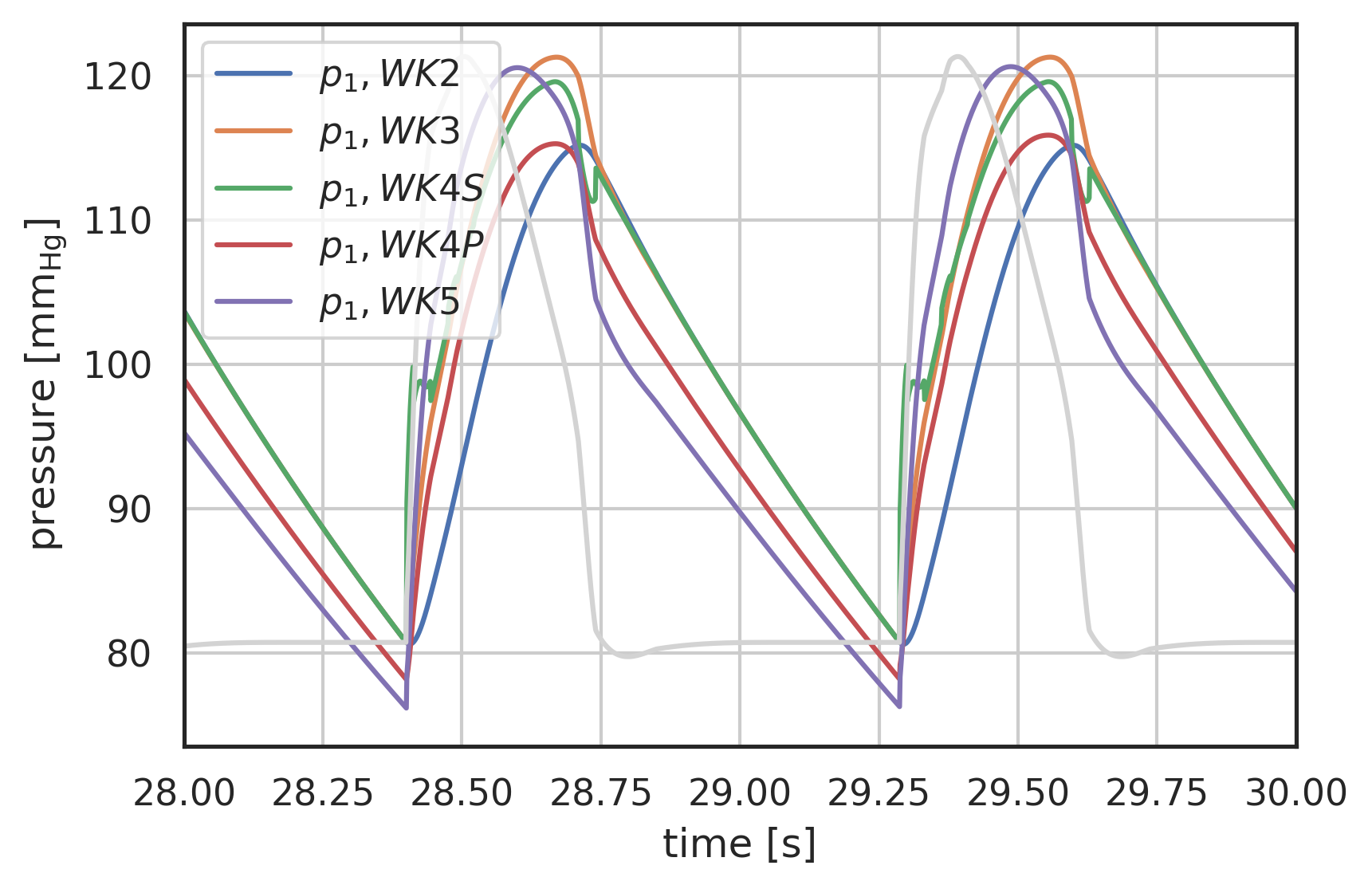
Figure 10: Pressure response to coarse scan input waveform, comparison of 2-Element (WK2), 3-Element (WK3) and 4-Element Windkessel models (WK4S - serial, WK4P - parallel), 5-element windkessel in this graph has Ls set to zero, so collapses to the parallel 4-element windkessel model.

Note: As can be seen from this graph, the serial 4-element WK is very sensitive to the inertance. Since in the current implementation this depends on $\frac{d^{2}I}{dt^{2}}$ it seems sensible to modify that implementation in a similar fashion as the 5-element model.

Note 2: Presumably the deviation between WK4P and WK5 has to do with the second flow derivative as well, and WK5 is therefore the better representation.

4 Validation of 3- and 4-element windkessel models

The validation uses data from [Stergiopulos1999a] Fig 4, type C. Flow and pressure waveforms for aortic flow. Data digitised using Engauge.

Read data in and arrange in vol array in the form that the windkessel module understands (unpack=True):

import numpy as np
import scipy as sp
import scipy.interpolate
import matplotlib.pyplot as plt
import lmfit

import windkessel as wk

datafile = "/home/thor/Documents/Research/stergiopulos1999_fig4_typeC.csv"

vol = np.genfromtxt(datafile, delimiter=",", skip_header=1, unpack=True)


datafile = "/home/thor/Documents/Research/stergiopulos1999_fig4_typeC_p.csv"

p = np.genfromtxt(datafile, delimiter=",", skip_header=1, unpack=True)

Define the inlet waveform function using the piecewise B-Spline wk.PWBezier:

def I_Stergio(t):
    return wk.PWBezier(vol, t)

plt.plot(vol[0], vol[1] / np.max(vol[1]), label="normalised volume flow")

plt.plot(
    p[0],
    (p[1] - np.min(p[1])) / (np.max(p[1]) - np.min(p[1])),
    label="normalised pulse pressure",
)

t = np.linspace(0, 0.8, 800)

plt.plot(t, I_Stergio(t) / np.max(vol[1]), "--", label="Bezier Approx", color="grey")

plt.legend()
plt.grid()

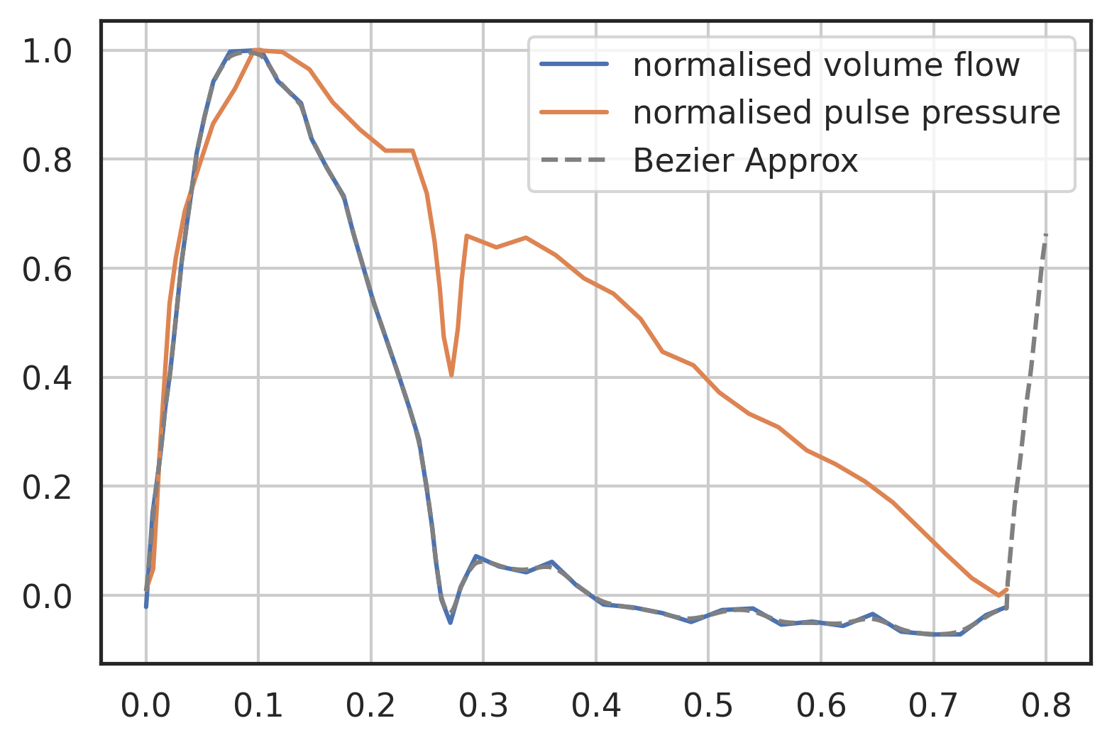
Figure 11: Measured flow rate and pulse pressure, data from [Stergiopulos1999a], Figure 4, type C aortic flow

The values for the windkessel models have been taken from [Stergiopulos1999a], table 2.

# Set parameters for Windkessel Model
# cite:Stergiopulos1999a Type C
Rc3 = 0.03
Rc4 = 0.045
Rp = 0.63
C3 = 5.16
C4 = 2.53
Lp = 0.0054
Ls = 0.0
# Rc3 = 0.03121307
# Rp3 = 0.63543930
# C3 =  4.54903588

time_start = 0
time_end = 10
N = (time_end - time_start) * 1000

Solve 3-element windkessel:

%time pressure3wk = wk.solve_wk(fun=I_Stergio, Rc=Rc3, Rp=Rp, C=C3, L=0.0, time_start=time_start, time_end=time_end, N=N, method="RK23", initial_cond=[0, 0], rtol=1e-8)

And the 4-element windkessel using the WK5 implementation with $L_{s} = 0$:

%time pressure4wk = wk.solve_wk5(fun=I_Stergio, Rc=Rc4, Rp=Rp, C=C4, Lp=Lp, Ls=0.0, time_start=time_start, time_end=time_end, N=N, method="RK23", initial_cond=[0, 0], rtol=1e-8)

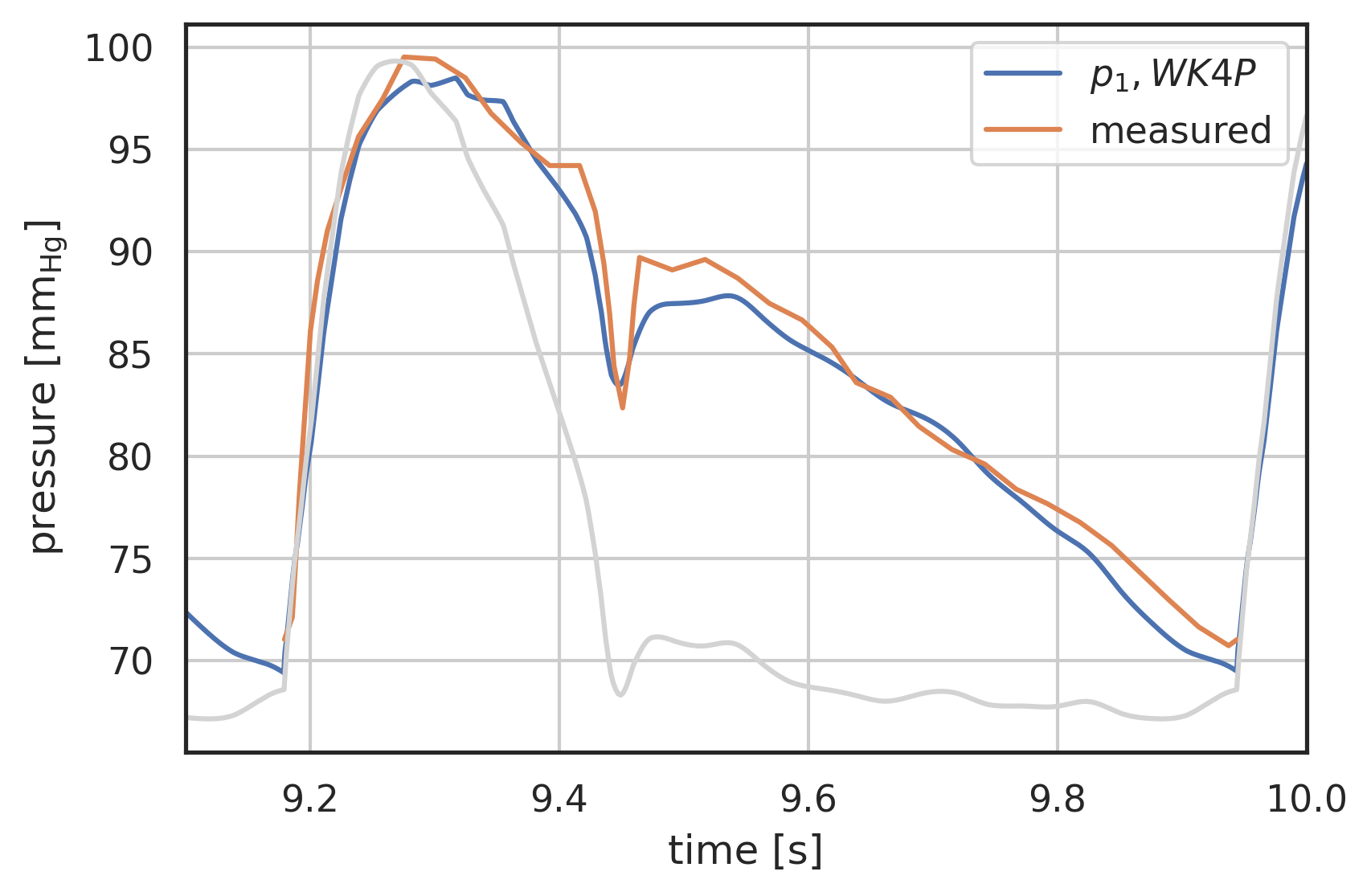
# plot curves
plt.xlabel("time [s]")
plt.ylabel("pressure [$\\mathrm{mm_{Hg}}$]")

startN = int(0.7 * N)
# plot first and second component (index 0, 1) of array 'y'
# over array 't':
# plt.plot(pressure2wk.t[startN:], pressure2wk.y[0][startN:], label="$p_1, WK2$")
#plt.plot(pressure3wk.t[startN:], pressure3wk.y[0][startN:], label="$p_1, WK3$")
# plt.plot(pressure4wks.t[startN:], pressure4wks.y[0][startN:], label="$p_1, WK4S$")
plt.plot(pressure4wk.t[startN:], pressure4wk.y[0][startN:], label="$p_1, WK4P$")
# plt.plot(
#     pressure.t[startN:],
#     pressure.y[0][startN:]
#     - R1 * I_generic(pressure.t[startN:])
#     - L * wk.ddt(I_generic, pressure.t[startN:]),
#     label="p_2 analytical",
# )

plt.plot(p[0] + 12 * np.max(vol[0]), p[1], label="measured")


t = np.linspace(8, 10, 1000)
plt.plot(
    t,
    I_Stergio(t)
    / np.max(I_Stergio(t))
    * (np.max(pressure3wk.y[0]) - np.min(pressure3wk.y[0][startN:]))
    + np.min(pressure3wk.y[0][startN:]),
    color="lightgrey",
)

plt.legend()
plt.grid()
plt.xlim(9.1, 10)

9.1

10.0

5 Parameter optimisation

One of the common problems is finding the parameters for a windkessel model based on measured flow rate and pressure waveforms.

This is an optimisation problem, similar to a curve fitting problem. In our case the model function is not given as a function, but as the integration problem solved above.

So let’s see if I can estimate the parameters for the windkessel models given volume flow rate and pressure measurements.

The easiest and most common way to fit a curve is using the Levenberg-Marquardt (LM) least-spares method. However in our case this fails. Most likely because the method cannot find clear derivates, or trends, based on the initial small shifts from the initial guess. It is also notorious for only finding local minima.

There are two scipy modules that are commonly used for these optimisation fits. The simply one is scipy.optimise, which will be sufficient in most cases. Then there is the lmfit framework (lmfit website), which has a few nice feature (a Model and Minimizer class, and the definition of parameters as a dictionary). lmfit also has some additional optimization routines (despite the name, it can do a lot more than LM).

This is the output of the LM least-squares fit. The result is always only very slightly different from the initial guess. So the LM method is not suitable for our problem, because it cannot establish a clear gradient from the initial guess.

[[Fit Statistics]]
    # fitting method   = leastsq
    # function evals   = 57
    # data points      = 45
    # variables        = 3
    chi-square         = 5737.26944
    reduced chi-square = 136.601653
    Akaike info crit   = 224.163428
    Bayesian info crit = 229.583416
[[Variables]]
    Rc:  0.02495009 +/- 0.01126909 (45.17%) (init = 1)
    Rp:  2.00057905 +/- 7.4233e-06 (0.00%) (init = 2)
    C:   9.99369127 +/- 4.7524e-04 (0.00%) (init = 10)
[[Correlations]] (unreported correlations are < 0.100)
    C(Rp, C)  = -0.906
    C(Rc, Rp) =  0.814
    C(Rc, C)  = -0.713

Note: I am not an expert in optimisation methods, so will need to invest some time in this. I will also need some help from somebody with more experience in this.

5.1 Monte Carlo Method

An obvious method to find a global minimum on any model would be the brute force method, i.e. scanning the whole parameter space with a given step. Obviously this scales with $N^{n}$, with $N$, number of scanning points, and $n$, number of parameters, which makes the method not economic and increasingly unsuitable with increasing number of parameters. It may be a solution in cases where the initial guess is relieable and the parameter space can be limited using a-priori knowledge.

lmfit has the Markov Chain Monte Carlo method as one of the optimisation frameworks. This integrates emcee to do the scanning of the parameter space. The parameter fit using this method seems to be reliable, but it is also scaling with $ ^{n}$ and is resource-hungry, if not parameterised close to the minimum.

The following code will run approx. 50 hours on a single CPU (2.5 GHz 5th gen i7), so is not implemented as a workbook, but as a standalone script:

Note: The script should parallelise, but doesn’t properly. The first iterations do spawn the child processed, but after the first 100 iteration (when the method is reinitialised for the second set - showing progress), it does not respawn the child processes and continues the run on a single CPU.

import numpy as np
import scipy as sp
import scipy.interpolate
import scipy.optimize
import matplotlib.pyplot as plt
import lmfit

import emcee
import windkessel as wk

# Import shared memory MP framework
# for distributed MPI use the "Schwimmbad" implementation of "Pool"
import multiprocessing

# Initialise the MP pool (shared memory on 28cpu node)
pool = multiprocessing.Pool(processes=28)


# Read data
datafile = "stergiopulos1999_fig4_typeC.csv"

vol = np.genfromtxt(datafile, delimiter=",", skip_header=1, unpack=True)


datafile = "stergiopulos1999_fig4_typeC_p.csv"

p = np.genfromtxt(datafile, delimiter=",", skip_header=1, unpack=True)


# Def volume flow waveform for windkessel model
def I_Stergio(t):
    return wk.PWBezier(vol, t)


# Function that will be optimised (Minimisation problem, so return residual)
def wk_residual(pars, t, data=None, eps=None):

    # unpack parameters: extract .value attribute for each parameter
    # 3-element windkessel
    parvals = pars.valuesdict()
    Rc = parvals["Rc"]
    Rp = parvals["Rp"]
    C = parvals["C"]
    # for 4/5 element use these:
    # Ls = parvals["Ls"]
    # Lp = parvals["Lp"]

    # 3-element, change for 4/5 element
    pressure = wk.solve_wk(
    # pressure = wk.solve_wk5(
        fun=I_Stergio,
        Rc=Rc,
        Rp=Rp,
        C=C,
        # 3-element wk, use the next line:
        L = 0.0;
        # 4/5 element, uncomment the following two lines:
        # Ls=Ls,
        # Lp=Lp,
        time_start=0,
        time_end=10,
        N=10000,
        method="RK45",
        initial_cond=[0, 0],
        rtol=1e-9,
    )

    # return the 11th cycle for optimisation
    t = t + 10 * np.max(t)

    # not really needed, but nice to keep an eye on the values and learn
    # how the algorithm develops the random walk
    print("Iteration values :", Rc, Rp, C)

    model = sp.interpolate.interp1d(
        pressure.t, pressure.y[0], fill_value="extrapolate"
    )(t)

    # return values or residual
    if data is None:
        return model
    if eps is None:
        return model - data
    return (model - data) / eps

# Main code starts here

# Initial values
Rc0 = 0.1
Rp0 = 2
C0 = 2.1
# for 4/5 element WK use the following:
# Ls0 = 0.02
# Lp0 = 0.02

# use times from the original scan data
t = p[0]


params = lmfit.Parameters()
params.add("Rc", value=Rc0, min=0.0, max=1.0)
params.add("Rp", value=Rp0, min=0.01, max=5.0)
params.add("C", value=C0, min=0.0, max=10.0)
# 4/5 wk:
# params.add("Ls", value=Ls0, min=0.0, max=1.0)
# params.add("Lp", value=Lp0, min=0.0001, max=1.0)


# call the minimizer
result = lmfit.minimize(
    wk_residual, params, args=(t, p[1]), method="emcee", workers=pool
)

# print result
print(lmfit.fit_report(result))

The result of this run is:

The chain is shorter than 50 times the integrated autocorrelation time for 3 parameter(s). Use this estimate with caution and run a longer chain!
N/50 = 20;
tau: [53.98102615 80.97150882 93.43245913]
Iteration values : 0.031213074384297365 0.6354393031093962 4.54903588439194
[[Fit Statistics]]
    # fitting method   = emcee
    # function evals   = 100000
    # data points      = 45
    # variables        = 3
    chi-square         = 280.230757
    reduced chi-square = 6.67216088
    Akaike info crit   = 88.3027908
    Bayesian info crit = 93.7227782
[[Variables]]
    Rc:  0.03121307 +/- 0.00108606 (3.48%) (init = 0.1)
    Rp:  0.63543930 +/- 0.19441108 (30.59%) (init = 2)
    C:   4.54903588 +/- 0.19736334 (4.34%) (init = 2.1)
[[Correlations]] (unreported correlations are < 0.100)
    C(Rp, C) =  0.537
    C(Rc, C) = -0.440

These values are close to the original optimisation in [Stergiopulos1999a]: $R_{c} = 0.03, R_{p} = 0.63, C = 5.16$. The resistances are within round-off, but the capacitance is $12\%$ lower.

Rc = 0.03121307
Rp = 0.63543930
C = 4.54903588

pressure3fitEMCEE = wk.solve_wk(
    fun=I_Stergio,
    Rc=Rc,
    Rp=Rp,
    C=C,
    L=0.0,
    time_start=time_start,
    time_end=time_end,
    N=N,
    method="RK45",
    initial_cond=[0, 0],
    rtol=1e-9,
)

# plot curves
plt.xlabel("time [s]")
plt.ylabel("pressure [$\\mathrm{mm_{Hg}}$]")

startN = int(0.7 * N)
# plot first and second component (index 0, 1) of array 'y'
# over array 't':
# plt.plot(pressure2wk.t[startN:], pressure2wk.y[0][startN:], label="$p_1, WK2$")
plt.plot(pressure3wk.t[startN:], pressure3wk.y[0][startN:], label="$p_1, WK3\ Stergiopulos\ fit$")
# plt.plot(pressure4wks.t[startN:], pressure4wks.y[0][startN:], label="$p_1, WK4S$")
plt.plot(pressure3fitEMCEE.t[startN:], pressure3fitEMCEE.y[0][startN:], label="$p_1, WK3\ EMCEE\ fit$")

# plt.plot(pressure4fitNM.t[startN:], pressure4fitNM.y[0][startN:], label="$p_1, WK4\ NM\ fit$")
# plt.plot(pressure5fitNM.t[startN:], pressure5fitNM.y[0][startN:], label="$p_1, WK5\ NM\ fit$")
# plt.plot(
#     pressure.t[startN:],
#     pressure.y[0][startN:]
#     - R1 * I_generic(pressure.t[startN:])
#     - L * wk.ddt(I_generic, pressure.t[startN:]),
#     label="p_2 analytical",
# )

plt.plot(p[0] + 12 * np.max(vol[0]), p[1], label="measured")


t = np.linspace(8, 10, 1000)
plt.plot(
    t,
    I_Stergio(t) / np.max(I_Stergio(t))
    *(np.max(pressure3wk.y[0]) - np.min(pressure3wk.y[0][startN:]))
    + np.min(pressure3wk.y[0][startN:]),
    color="lightgrey",
)

plt.legend()
plt.grid()
plt.xlim(9.1, 10);

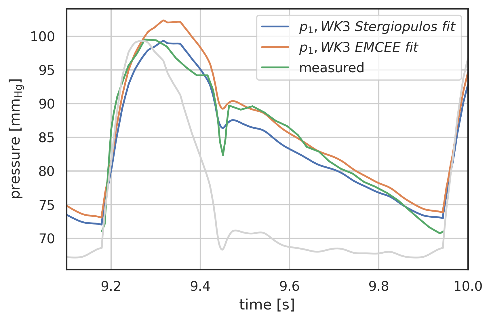
Figure 13: Parameter Optimisation for 3-element windkessel, EMCEE optimisation compared to parameters from [Stergiopulos1999a]

Note: This is promising and shows that the parameter optimisation is working. But there must be a better algorithm for this. Or at least a way to get the parameter scanning work in parallel.

5.1.1 TODO Run local minimum scan

Based on this result a localised scan in a 20% window around the values found in the first run is running. The hope is, that a two staged approach will prove to be more accurate and scale better.

5.1.2 TODO 4/5 element windkessel optimisation

Running at the moment, estimated wallclock time for single CPU run: 520 hours

5.2 Nelder-Mead Optimisation

Matlab’s standard fitting tool fminsearch uses the Nelder-Mead Method (NM) to optimise the parameters. NM is a gradient free optimiser for local minima. So it depends on a good initial guess. But it is efficient and a lot quicker than the Monte Carlo method (12 minutes vs 50 hours for the 3-element optimisation).

3- element optimisation, runtime 12 minutes, single CPU:

[[Fit Statistics]]
    # fitting method   = Nelder-Mead
    # function evals   = 381
    # data points      = 45
    # variables        = 3
    chi-square         = 279.735389
    reduced chi-square = 6.66036640
    Akaike info crit   = 88.2231732
    Bayesian info crit = 93.6431607
[[Variables]]
    Rc:  0.03113800 +/- 0.00154258 (4.95%) (init = 0.1)
    Rp:  0.63460135 +/- 0.00196631 (0.31%) (init = 1)
    C:   4.54947360 +/- 0.01356166 (0.30%) (init = 2.1)
[[Correlations]] (unreported correlations are < 0.100)
    C(Rc, Rp) = -0.353

So the Nelder-Mead optimisation arrives at the same solution than the MC method, but at a significantly lower computational cost (381 integration runs for NM, 100000 integration runs for MC).

4-element opimisation, parallel inertance, runtime 75 minutes, single CPU:

[[Fit Statistics]]
    # fitting method   = Nelder-Mead
    # function evals   = 743
    # data points      = 45
    # variables        = 4
    chi-square         = 166.525129
    reduced chi-square = 4.06158851
    Akaike info crit   = 66.8817679
    Bayesian info crit = 74.1084179
[[Variables]]
    Rc:  0.04315254 +/- 4.4396e-04 (1.03%) (init = 0.1)
    Rp:  0.63486371 +/- 0.00142771 (0.22%) (init = 1)
    C:   2.39246377 +/- 0.01014358 (0.42%) (init = 2.1)
    Lp:  0.00536603 +/- 5.1957e-05 (0.97%) (init = 0.02)
[[Correlations]] (unreported correlations are < 0.100)
    C(C, Lp) = -0.163
    C(Rp, C) = -0.156
    C(Rc, C) = -0.143

These values are very close to the original optimisation in [Stergiopulos1999a]: $R_{c} = 0.043, R_{p} = 0.63, C = 2.53, L_{p} = 0.0054$. Capacitance is again estimated lower here, but the effect is less obvious in the pressure waveform:

Note: The 4-element optimisation with serial inertance converges to the same values as the 3-element optimisation with an extremely low inertance:

4-element opimisation, serial inertance, runtime 20 minutes, single CPU:

[[Fit Statistics]]
    # fitting method   = Nelder-Mead
    # function evals   = 578
    # data points      = 45
    # variables        = 4
    chi-square         = 279.534545
    reduced chi-square = 6.81791574
    Akaike info crit   = 90.1908526
    Bayesian info crit = 97.4175026
[[Variables]]
    Rc:  0.03112870 +/- 0.00146585 (4.71%) (init = 0.1)
    Rp:  0.63447718 +/- 7.9329e-04 (0.13%) (init = 1)
    C:   4.54515385 +/- 0.00544312 (0.12%) (init = 2.1)
    Ls:  7.6397e-10 +/- 2.8473e-07 (37269.54%) (init = 0.02)
[[Correlations]] (unreported correlations are < 0.100)
    C(Rc, Rp) = -0.101

5-element optimisation, runtime 90 minutes, single CPU:

[[Fit Statistics]]
    # fitting method   = Nelder-Mead
    # function evals   = 916
    # data points      = 45
    # variables        = 5
    chi-square         = 166.517988
    reduced chi-square = 4.16294969
    Akaike info crit   = 68.8798381
    Bayesian info crit = 77.9131506
[[Variables]]
    Rc:  0.04306403 +/- 4.1288e-04 (0.96%) (init = 0.1)
    Rp:  0.63485549 +/- 0.00129126 (0.20%) (init = 1)
    C:   2.39128343 +/- 0.00666945 (0.28%) (init = 1)
    Ls:  1.5358e-05 +/- 2.6904e-06 (17.52%) (init = 0.02)
    Lp:  0.00535077 +/- 5.4970e-05 (1.03%) (init = 0.02)
[[Correlations]] (unreported correlations are < 0.100)
    C(C, Lp)  =  0.412
    C(Ls, Lp) =  0.308

5.2.1 Comparison of 3-, 4-, and 5-element windkessel models with Nelder-Mead optimised parameters. ATTACH

Rc = 0.03121307
Rp = 0.63543930
C = 4.54903588

pressure3fitNM = wk.solve_wk(
    fun=I_Stergio,
    Rc=Rc,
    Rp=Rp,
    C=C,
    L=0.0,
    time_start=time_start,
    time_end=time_end,
    N=N,
    method="RK45",
    initial_cond=[0, 0],
    rtol=1e-9,
)

Rc = 0.04315254
Rp = 0.63486371
C = 2.39246377
Lp = 0.00536603

pressure4fitNM = wk.solve_wk5(
    fun=I_Stergio,
    Rc=Rc,
    Rp=Rp,
    C=C,
    Lp=Lp,
    Ls=0.0,
    time_start=time_start,
    time_end=time_end,
    N=N,
    method="RK45",
    initial_cond=[0, 0],
    rtol=1e-9,
)

Rc =  0.04306403
Rp =  0.63485549
C =  2.39128343
Ls =  1.5358e-05
Lp =  0.00535077

pressure5fitNM = wk.solve_wk5(
    fun=I_Stergio,
    Rc=Rc,
    Rp=Rp,
    C=C,
    Ls=Ls,
    Lp=Lp,
    time_start=time_start,
    time_end=time_end,
    N=N,
    method="RK45",
    initial_cond=[0, 0],
    rtol=1e-9,
)

# plot curves
plt.xlabel("time [s]")
plt.ylabel("pressure [$\\mathrm{mm_{Hg}}$]")

startN = int(0.7 * N)
# plot first and second component (index 0, 1) of array 'y'
# over array 't':
# plt.plot(pressure2wk.t[startN:], pressure2wk.y[0][startN:], label="$p_1, WK2$")
plt.plot(
    pressure3wk.t[startN:],
    pressure3wk.y[0][startN:],
    label="$p_1, WK3\ Stergiopulos\ fit$",
)
# plt.plot(pressure4wks.t[startN:], pressure4wks.y[0][startN:], label="$p_1, WK4S$")
# plt.plot(pressure3fitEMCEE.t[startN:], pressure3fitEMCEE.y[0][startN:], label="$p_1, WK3\ EMCEE\ fit$")
plt.plot(
    pressure3fitNM.t[startN:], pressure3fitNM.y[0][startN:], label="$p_1, WK3\ NM\ fit$"
)
plt.plot(
    pressure4fitNM.t[startN:], pressure4fitNM.y[0][startN:], label="$p_1, WK4\ NM\ fit$"
)

plt.plot(
    pressure5fitNM.t[startN:],
    pressure5fitNM.y[0][startN:],
    "--",
    label="$p_1, WK5\ NM\ fit$",
)
# plt.plot(
#     pressure.t[startN:],
#     pressure.y[0][startN:]
#     - R1 * I_generic(pressure.t[startN:])
#     - L * wk.ddt(I_generic, pressure.t[startN:]),
#     label="p_2 analytical",
# )

plt.plot(p[0] + 12 * np.max(vol[0]), p[1], "k--", label="measured")


t = np.linspace(8, 10, 1000)
plt.plot(
    t,
    I_Stergio(t)
    / np.max(I_Stergio(t))
    * (np.max(pressure3wk.y[0]) - np.min(pressure3wk.y[0][startN:]))
    + np.min(pressure3wk.y[0][startN:]),
    color="lightgrey",
)

plt.legend()
plt.grid()
plt.xlim(9.1, 10);

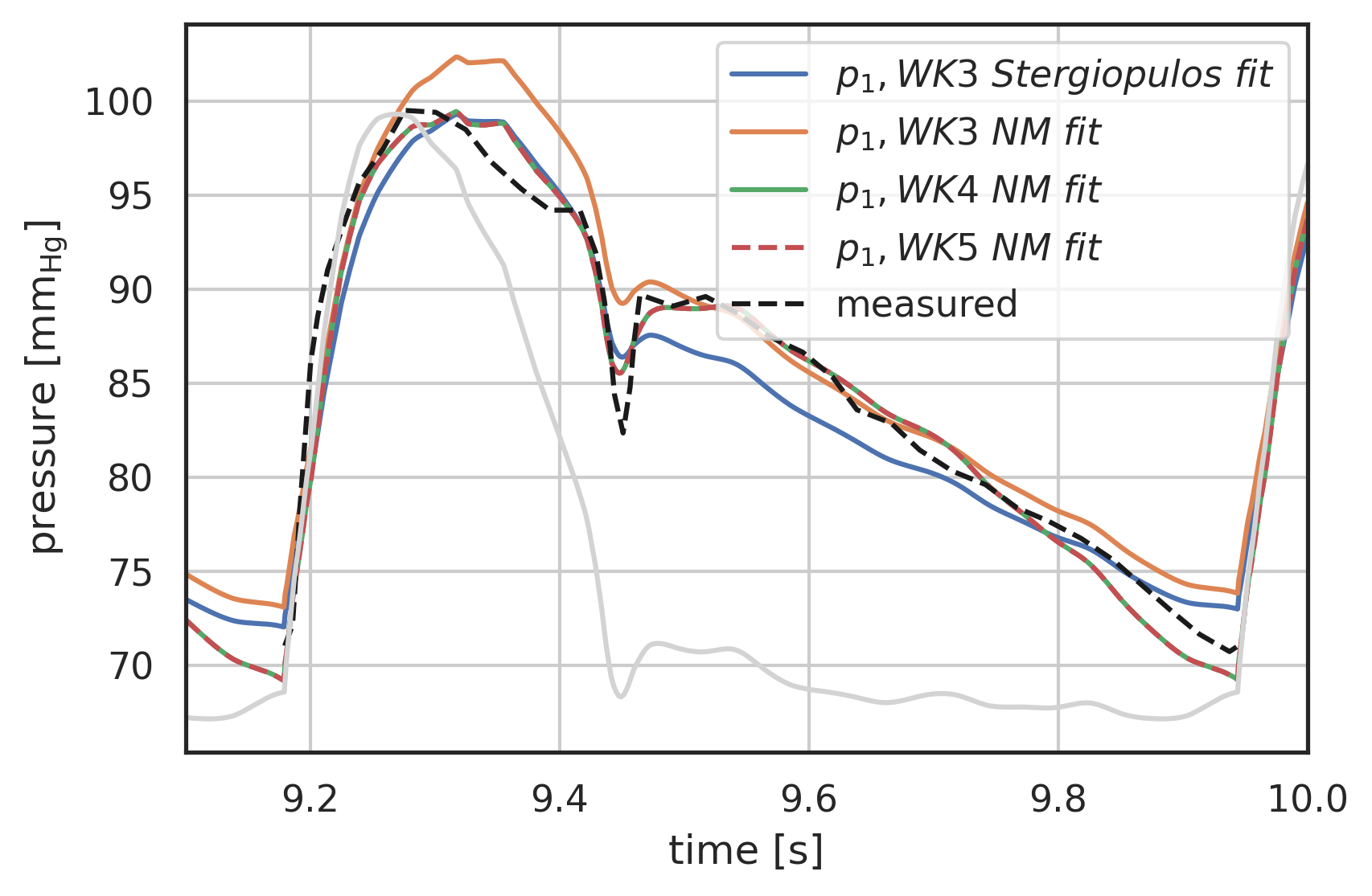
Figure 14: Parameter Optimisation for 3-, 4-, and 5-element windkessel, NM optimisation compared to measurement and 3-element fit from [Stergiopulos1999a]. 3-element NM is off and does not converge to the same capacitance as [Stergiopulos1999a]. 4-element parallel and 5-element windkessel model results are virtually identical.

Note: The 3-element windkessel optimisation does not find the same capacitance as in [Stergiopulos1999a]. The same occurs in the 4-element serial model. This needs further research.

Assumption: The 3-element windkessel is either too high during systole or too low during diastole. Since diastole is longer, its influence on the overall residual that is minimised is higher.

6 Bibliography

[Pedrizzetti1996] Pedrizzetti, Unsteady Tube Flow over an Expansion, Journal of Fluid Mechanics 310, 89-111 (1996).
[Schenkel2009] Schenkel, Malve, Reik, Markl, Jung & Oertel, MRI-Based CFD Analysis of Flow in a Human Left Ventricle: Methodology and Application to a Healthy Heart., Annals of Biomedical Engineering 37(3), 503-515 (2009).
[Stergiopulos1999a] Stergiopulos, Westerhof & Westerhof, Total Arterial Inertance as the Fourth Element of the Windkessel Model, American Journal of Physiology-Heart and Circulatory Physiology 276(1), H81-H88 (1999).

Footnotes:

… intended to be a package comprising all of the tools I use for physiological flow models

Never use the import * from method, this will cause functions to be overwritten and makes for code that is terrible to read and impossible to debug

Windkessel Python Module

Table of Contents

1 Derivation of windkessel equations

1.1 2-Element Windkessel model (wk2)

1.2 3-Element Windkessel model (wk3) and 4-element Windkessel model with serial impedance (wk4s)

1.2.1 Alternative implementation in \(P_{2}\) without \(\frac{d^{2}I}{dt^{2}}\)

1.3 4-Element Windkessel model - parallel (wk4p)

1.4 5-Element Windkessel model - parallel and serial inductance (wk5)

2 Python module

2.1 Windkessel Models

2.1.1 TODO reformulate without \(\frac{d^{2}I}{dt^{2}}\)

2.2 Waveform Approximation

3 Using the module

3.1 Importing all the necessary modules

3.2 Setting the input waveform

3.2.1 Generic sine based waveform with dicrotic notch

3.3 Solving the windkessel equations

3.4 Pedrizzetti waveform [Pedrizzetti1996]

3.5 TODO Working with high temporal resolution volume flow data

3.5.1 TODO FFT/IFFT implementation

3.6 Working with low temporal resolution scanned volume flow data

4 Validation of 3- and 4-element windkessel models

5 Parameter optimisation

5.1 Monte Carlo Method

5.1.1 TODO Run local minimum scan

5.1.2 TODO 4/5 element windkessel optimisation

5.2 Nelder-Mead Optimisation

5.2.1 Comparison of 3-, 4-, and 5-element windkessel models with Nelder-Mead optimised parameters. ATTACH

6 Bibliography

Footnotes: