# # Importing the required packages

using CirculatorySystemModels
using ModelingToolkit
using OrdinaryDiffEqVerner
using Plots
using DisplayAs
A simple single-chamber model
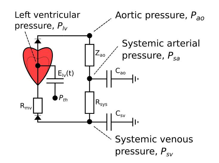
This follows Bjørdalsbakke et al.
Bjørdalsbakke, N.L., Sturdy, J.T., Hose, D.R., Hellevik, L.R., 2022. Parameter estimation for closed-loop lumped parameter models of the systemic circulation using synthetic data. Mathematical Biosciences 343, 108731. https://doi.org/10.1016/j.mbs.2021.108731
Changes from the published version above:
- Capacitors are replaced by compliances. These are identical to capacitors, but have an additional parameter, the unstrained volume $V_0$, which allows for realistic blood volume modelling. Compliances have an inlet and an oulet in line with the flow, rather than the ground connector of the dangling capacitor.
- The aortic resistor is combined with the valve (diode) in the
ResistorDiodeelement.
Define the parameters
All the parameters are taken from table 1 of [Bjørdalsbakke2022].
Cycle time in seconds
#
τ = 0.850.85Double Hill parameters for the ventricle
Eₘᵢₙ = 0.03
Eₘₐₓ = 1.5
n1LV    = 1.32;
n2LV    = 21.9;
Tau1fLV = 0.303 * τ;
Tau2fLV = 0.508 * τ
#0.4318Resistances and Compliances
R_s = 1.11
C_sa = 1.13
C_sv = 11.011.0Valve parameters
Aortic valve basic
Zao = 0.0330.033Mitral valve basic
Rmv = 0.006

# Inital Pressure (mean cardiac filling pressure)
MCFP = 7.0

### Calculating the additional `k` parameter7.0The ventricle elastance is modelled as:
\[E_{l v}(t)=\left(E_{\max }-E_{\min }\right) e(t)+E_{\min }\]
where $e$ is a double-Hill function, i.e., two Hill-functions, which are multiplied by each other:
\[e(\tau)= k \times \frac{\left(\tau / \tau_1\right)^{n_1}}{1+\left(\tau / \tau_1\right)^{n_1}} \times \frac{1}{1+\left(\tau / \tau_2\right)^{n_2}}\]
and $k$ is a scaling factor to assure that $e(t)$ has a maximum of $e(t)_{max} = 1$:
\[k = \max \left(\frac{\left(\tau / \tau_1\right)^{n_1}}{1+\left(\tau / \tau_1\right)^{n_1}} \times \frac{1}{1+\left(\tau / \tau_2\right)^{n_2}} \right)^{-1}\]
nstep = 1000
t = LinRange(0, τ, nstep)

kLV = 1 / maximum((t ./ Tau1fLV).^n1LV ./ (1 .+ (t ./ Tau1fLV).^n1LV) .* 1 ./ (1 .+ (t ./ Tau2fLV).^n2LV))1.6721792928965973Set up the model elements
Set up time as a variable t
@variables t1-element Vector{Symbolics.Num}:
tHeart is modelled as a single chamber (we call it LV for "Left Ventricle" so the model can be extended later, if required):
@named LV = DHChamber(V₀ = 0.0, Eₘₐₓ=Eₘₐₓ, Eₘᵢₙ=Eₘᵢₙ, n₁=n1LV, n₂=n2LV, τ = τ, τ₁=Tau1fLV, τ₂=Tau2fLV, k = kLV, Eshift=0.0)Model LV:
Subsystems (2): see hierarchy(LV)
in
out
Equations (6):
4 standard: see equations(LV)
2 connecting: see equations(expand_connections(LV))
Unknowns (6): see unknowns(LV)
V(t)
p(t)
in₊p(t)
in₊q(t)
⋮
Parameters (11): see parameters(LV)
V₀
p₀
Eₘᵢₙ
Eₘₐₓ
⋮The two valves are simple diodes with a small resistance (resistance is needed, since perfect diodes would connect two elastances/compliances, which will lead to unstable oscillations):
@named AV = ResistorDiode(R=Zao)
@named MV = ResistorDiode(R=Rmv)
Model MV:
Subsystems (2): see hierarchy(MV)
in
out
Equations (6):
4 standard: see equations(MV)
2 connecting: see equations(expand_connections(MV))
Unknowns (6): see unknowns(MV)
Δp(t)
q(t)
in₊p(t)
in₊q(t)
⋮
Parameters (1): see parameters(MV)
RThe main components of the circuit are 1 resistor Rs and two compliances for systemic arteries Csa, and systemic veins Csv (names are arbitrary). Note: one of the compliances is defined in terms of $dV/dt$ using the option inV = true. The other without that option is in $dp/dt$.
@named Rs = Resistor(R=R_s)

@named Csa = Compliance(C=C_sa)
@named Csv = Compliance(C=C_sv, inP=true)
Model Csv:
Subsystems (2): see hierarchy(Csv)
in
out
Equations (6):
4 standard: see equations(Csv)
2 connecting: see equations(expand_connections(Csv))
Unknowns (6): see unknowns(Csv)
V(t)
p(t)
in₊p(t)
in₊q(t)
⋮
Parameters (2): see parameters(Csv)
V₀
CBuild the system
Connections
The system is built using the connect function. connect sets up the Kirchhoff laws:
- pressures are the same in all connected branches on a connector
- sum of all flow rates at a connector is zero
The resulting set of Kirchhoff equations is stored in circ_eqs:
circ_eqs = [
    connect(LV.out, AV.in)
    connect(AV.out, Csa.in)
    connect(Csa.out, Rs.in)
    connect(Rs.out, Csv.in)
    connect(Csv.out, MV.in)
    connect(MV.out, LV.in)
]
6-element Vector{Symbolics.Equation}:
connect(Model LV.out:
Equations (2):
2 connecting: see equations(expand_connections(LV.out))
Unknowns (2): see unknowns(LV.out)
p(t)
q(t), Model AV.in:
Equations (2):
2 connecting: see equations(expand_connections(AV.in))
Unknowns (2): see unknowns(AV.in)
p(t)
q(t))
connect(Model AV.out:
Equations (2):
2 connecting: see equations(expand_connections(AV.out))
Unknowns (2): see unknowns(AV.out)
p(t)
q(t), Model Csa.in:
Equations (2):
2 connecting: see equations(expand_connections(Csa.in))
Unknowns (2): see unknowns(Csa.in)
p(t)
q(t))
connect(Model Csa.out:
Equations (2):
2 connecting: see equations(expand_connections(Csa.out))
Unknowns (2): see unknowns(Csa.out)
p(t)
q(t), Model Rs.in:
Equations (2):
2 connecting: see equations(expand_connections(Rs.in))
Unknowns (2): see unknowns(Rs.in)
p(t)
q(t))
connect(Model Rs.out:
Equations (2):
2 connecting: see equations(expand_connections(Rs.out))
Unknowns (2): see unknowns(Rs.out)
p(t)
q(t), Model Csv.in:
Equations (2):
2 connecting: see equations(expand_connections(Csv.in))
Unknowns (2): see unknowns(Csv.in)
p(t)
q(t))
connect(Model Csv.out:
Equations (2):
2 connecting: see equations(expand_connections(Csv.out))
Unknowns (2): see unknowns(Csv.out)
p(t)
q(t), Model MV.in:
Equations (2):
2 connecting: see equations(expand_connections(MV.in))
Unknowns (2): see unknowns(MV.in)
p(t)
q(t))
connect(Model MV.out:
Equations (2):
2 connecting: see equations(expand_connections(MV.out))
Unknowns (2): see unknowns(MV.out)
p(t)
q(t), Model LV.in:
Equations (2):
2 connecting: see equations(expand_connections(LV.in))
Unknowns (2): see unknowns(LV.in)
p(t)
q(t))Add the component equations
In a second step, the system of Kirchhoff equations is completed by the component equations (both ODEs and AEs), resulting in the full, overdefined ODE set circ_model.
Note: we do this in two steps.
@named _circ_model = ODESystem(circ_eqs, t)

@named circ_model = compose(_circ_model,
                          [LV, AV, MV, Rs, Csa, Csv])
Model circ_model:
Subsystems (6): see hierarchy(circ_model)
LV
AV
MV
Rs
⋮
Equations (42):
30 standard: see equations(circ_model)
12 connecting: see equations(expand_connections(circ_model))
Unknowns (36): see unknowns(circ_model)
LV₊V(t)
LV₊p(t)
LV₊in₊p(t)
LV₊in₊q(t)
⋮
Parameters (18): see parameters(circ_model)
LV₊V₀
LV₊p₀
LV₊Eₘᵢₙ
LV₊Eₘₐₓ
⋮Simplify the ODE system
The crucial step in any acausal modelling is the sympification and reduction of the OD(A)E system to the minimal set of equations. ModelingToolkit.jl does this in the structural_simplify function.
circ_sys = structural_simplify(circ_model)Model circ_model:
Equations (3):
3 standard: see equations(circ_model)
Unknowns (3): see unknowns(circ_model)
Csv₊in₊p(t)
Csa₊V(t)
LV₊V(t)
Parameters (18): see parameters(circ_model)
LV₊V₀
LV₊p₀
LV₊Eₘᵢₙ
LV₊Eₘₐₓ
⋮
Observed (33): see observed(circ_model)circ_sys is now the minimal system of equations. In this case it consists of 3 ODEs for the ventricular volume and the systemic and venous pressures.
Note: this reduces and optimises the ODE system. It is, therefore, not always obvious, which states it will use and which it will drop. We can use the states and observed function to check this. It is recommended to do this, since small changes can reorder states, observables, and parameters.
States in the system are now:
unknowns(circ_sys)3-element Vector{SymbolicUtils.BasicSymbolicImpl.var"typeof(BasicSymbolicImpl)"{SymbolicUtils.SymReal}}:
Csv₊in₊p(t)
Csa₊V(t)
LV₊V(t)Observed variables - the system will drop these from the ODE system that is solved, but it keeps all the algebraic equations needed to calculate them in the system object, as well as the ODEProblem and solution object - are:
observed(circ_sys)33-element Vector{Symbolics.Equation}:
Csa₊in₊p(t) ~ (-Csa₊V₀ + Csa₊V(t)) / Csa₊C
LV₊in₊p(t) ~ LV₊p₀ + (LV₊Eₘᵢₙ + ((-LV₊Eₘᵢₙ + LV₊Eₘₐₓ)*LV₊k*((rem(t + (1 - LV₊Eshift)*LV₊τ, LV₊τ) / LV₊τ₁)^LV₊n₁)) / ((1 + (rem(t + (1 - LV₊Eshift)*LV₊τ, LV₊τ) / LV₊τ₁)^LV₊n₁)*(1 + (rem(t + (1 - LV₊Eshift)*LV₊τ, LV₊τ) / LV₊τ₂)^LV₊n₂)))*(-LV₊V₀ + LV₊V(t))
Csv₊p(t) ~ Csv₊in₊p(t)
Rs₊out₊p(t) ~ Csv₊in₊p(t)
Csv₊out₊p(t) ~ Csv₊in₊p(t)
MV₊in₊p(t) ~ Csv₊in₊p(t)
Csv₊V(t) ~ Csv₊V₀ + Csv₊C*Csv₊in₊p(t)
Rs₊Δp(t) ~ -Csa₊in₊p(t) + Csv₊in₊p(t)
Csa₊p(t) ~ Csa₊in₊p(t)
AV₊out₊p(t) ~ Csa₊in₊p(t)
⋮
MV₊in₊q(t) ~ (-MV₊Δp(t)*(MV₊Δp(t) < 0)) / MV₊R
AV₊out₊q(t) ~ -AV₊in₊q(t)
LV₊out₊q(t) ~ -AV₊in₊q(t)
AV₊q(t) ~ AV₊in₊q(t)
Csa₊in₊q(t) ~ AV₊in₊q(t)
MV₊q(t) ~ MV₊in₊q(t)
Csv₊out₊q(t) ~ -MV₊in₊q(t)
LV₊in₊q(t) ~ MV₊in₊q(t)
MV₊out₊q(t) ~ -MV₊in₊q(t)And the parameters (these could be reordered, so check these, too):
parameters(circ_sys)18-element Vector{SymbolicUtils.BasicSymbolicImpl.var"typeof(BasicSymbolicImpl)"{SymbolicUtils.SymReal}}:
LV₊V₀
LV₊p₀
LV₊Eₘᵢₙ
LV₊Eₘₐₓ
LV₊n₁
LV₊n₂
LV₊τ
LV₊τ₁
LV₊τ₂
LV₊k
LV₊Eshift
AV₊R
MV₊R
Rs₊R
Csa₊V₀
Csa₊C
Csv₊V₀
Csv₊CDefine the ODE problem
First defined initial conditions u0 and the time span for simulation:
Note: the initial conditions are defined as a parameter map, rather than a vector, since the parameter map allows for changes in order. This map can include not only state-variables, but also observables (like LV.p in this case), which makes setting up the initial conditions easier, if the known initial conditions are not included in the resulting model states, which is often the case in MTK models. Since MTK9 these cannot be redundant, however, so we need to decide if we want to define pressures or volumes in this case.
u0 = [
        LV.p => MCFP
        Csa.p => MCFP
        Csv.p => MCFP
        ]
3-element Vector{Pair{Symbolics.Num, Float64}}:
LV₊p(t) => 7.0
Csa₊p(t) => 7.0
Csv₊p(t) => 7.0tspan = (0, 20)(0, 20)in this case we use the mean cardiac filling pressure as initial condition, and simulate 20 seconds.
Then we can define the problem:
prob = ODEProblem(circ_sys, u0, tspan)ODEProblem with uType Vector{Float64} and tType Int64. In-place: true
Initialization status: FULLY_DETERMINED
Non-trivial mass matrix: false
timespan: (0, 20)
u0: 3-element Vector{Float64}:
7.0
7.909999999999999
233.33333333333334Simulate
The ODE problem is now in the MTK/DifferentialEquations.jl format and we can use any DifferentialEquations.jl solver to solve it:
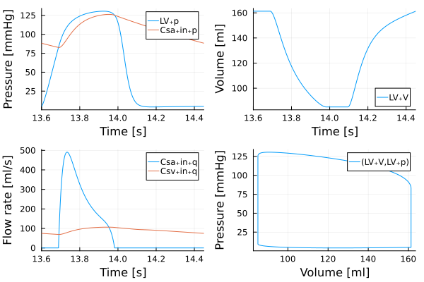
sol = solve(prob, Vern7(), reltol=1e-12, abstol=1e-12);Results
p1 = plot(sol, idxs=[LV.p,  Csa.in.p], tspan=(16 * τ, 17 * τ), xlabel = "Time [s]", ylabel = "Pressure [mmHg]",  hidexaxis = nothing) # Make a line plot
p2 = plot(sol, idxs=[LV.V], tspan=(16 * τ, 17 * τ),xlabel = "Time [s]", ylabel = "Volume [ml]",  linkaxes = :all)
p3 = plot(sol, idxs=[Csa.in.q,Csv.in.q], tspan=(16 * τ, 17 * τ),xlabel = "Time [s]", ylabel = "Flow rate [ml/s]", linkaxes = :all)
p4 = plot(sol, idxs=(LV.V, LV.p), tspan=(16 * τ, 17 * τ),xlabel = "Volume [ml]", ylabel = "Pressure [mmHg]", linkaxes = :all)

img = plot(p1, p2, p3, p4; layout=@layout([a b; c d]), legend = true)

img = DisplayAs.Text(DisplayAs.PNG(img))

img
#
This page was generated using Literate.jl.